Category Archives: Misconceptions

Post-publication review: Tournassat and Steefel (2015), part VI

This is the sixth and final (!) part of the review of “Ionic Transport in Nano-Porous Clays with Consideration of Electrostatic Effects” (Tournassat and Steefel (2015) (referred to as TS15 in the following). For background and context, please check the first part.

Recap

Let’s begin by reminding ourselves where we are in the “story” of the article. TS15 begun by vaguely suggesting that diffusion in bentonite1 cannot be modeled by assuming “Fickian” diffusion. The argument, however, is based on the inability of the traditional diffusion-sorption model to be reasonably fitted to ion through-diffusion data. This inability is not primarily due to assuming Fickian diffusion, but due to assuming immobility of the “sorbed” ions and due to assuming that the pore volume contains nothing but bulk water.

After being promised to be presented “fundamental properties” of bentonite that apparently will demonstrate the problem with assuming “Fickian” diffusion, we were instead introduced to a large set of modeling concepts. As a description of actual compacted bentonite, these concepts are mostly irrelevant (e.g. the Gouy-Chapman model), unjustified (e.g. Stern layers on basal surfaces), or simply fantasies (e.g. the idea of “stacks”, or the idea of Donnan equilibrium on the microscopic scale).

Finally, we were presented the Nernst-Planck approach to ion diffusion, which indeed goes beyond a Fickian description. The presented model, however, which includes “bulk water”, “diffuse layer” and “interlayer” domains assumed to be in equilibrium locally, is not suitable for compacted bentonite. Furthermore, no description whatsoever is presented for how this equilibrium is supposed to be maintained. The model is therefore incapable, even principally, to account for swelling — the most profound feature of bentonite in contact with an aqueous solution. Note also that discrimination between “diffuse layer” and “interlayer” domains is based on the pure fantasy of “stacks” as fundamental structural units.

We also showed that the presented Nernst-Planck framework was incorrectly derived, and after having sorted out how it can be reinterpreted,2 we noted that the suggested “concentration” and “diffusion potential” contributions to the diffuse layer flux where completely unfounded.

“From diffusive flux to diffusive transport equations”

In this section I expected to be given an overview of how all the previously introduced model components are supposed to fit together in an overall description for bentonite. With so many parts, there are a large number of quantities to consider. Apart from all the species concentrations in the different “porosity domains”, TS15 have also introduced e.g. electrostatic potentials (eqs. 17, 18, 21, 22, 39, 48, 56 in TS15), adsorption sites on “basal surfaces” (eq. 19 in TS15), “exchanger” sites (eq. 24 in TS15), “layer edge amphoteric” sites (eq. 28 in TS15), models for activity coefficients and their spatial derivatives (eqs. 58, 60, 64 in TS15), and entertained the possibility of having varying sizes of the “porosity domains” (although no constitutive relations has been stated).

Instead, the only thing related to a model description here is a restatement of the mass conservation law. This was already presented in eq. 4 in TS15, but is here incorrectly called the “diffusion equation” (TS15 eq. 65), and stated with an incorrect sign (TS15 eqs. 65, 66 and 68). TS15 express it in its final form as (I have here corrected the sign error, and suppressed an index \(i\))

\begin{equation} \frac{\partial}{\partial t} \left ( \phi_\mathrm{bulk}c_\mathrm{bulk} + \phi_\mathrm{DL}c_\mathrm{DL} + \phi_\mathrm{exch}c_\mathrm{exch} \right) = -\frac{\partial}{\partial x} \left ( j_\mathrm{bulk} + j_\mathrm{DL} + j_\mathrm{exch} \right ) \tag{1} \end{equation}

where \(\phi_\mathrm{bulk}\), \(\phi_\mathrm{DL}\) and \(\phi_\mathrm{exch}\) denotes the bulk water, “diffuse layer” and “interlayer” porosites, respectively; \(c_\mathrm{bulk}\), \(c_\mathrm{DL}\), \(c_\mathrm{exch}\) are the concentrations of the considered species in these “porosity domains”; and \(j_\mathrm{bulk}\), \(j_\mathrm{DL}\), and \(j_\mathrm{exch}\) are the corresponding domain fluxes (presumably given from the previously presented Nernst-Planck framework?).

That’s it.

As the authors stress the importance of adsorption processes throughout the article (even on montmorillonite basal surfaces), I find it very odd to here present an equation that completely omits them. Somewhat ironically, adsorption was included previously, in the section titled “Diffusion basics” (eq. 6 — 8 in TS15). Instead, the above equation (eq. 1) implies mechanisms that may alter the sizes of the “porosity domains” (i.e. \(d\phi/dt \neq 0\), \( d\phi/dx \neq 0 \)). But the article has not presented any constitutive relations for such mechanisms! This whole model presentation feels like having been handed a heap of irregular puzzle pieces with a promise of a grand result, while the reference photo belongs to a different puzzle.

Although eq. 1 provides little concrete information on the actual model, it still manages to contain a fatal flaw: the three domain fluxes are simply added to form some sort of a “total” flux. But this is not how diffusive fluxes work! The first real post I wrote on this blog covered this issue. There we noticed that domain fluxes are added in essentially all publications where multi-porous models are applied to bentonite. To see that separate domain fluxes are not additive should be as simple as considering some specific domain configuration. A trivial example is two domain types connected in series
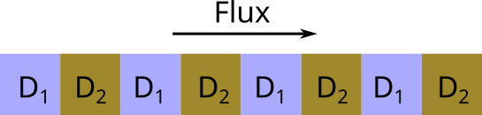
It is easy to see that the resulting flux in this case cannot be described as a sum of independent domain contributions (e.g, the flux vanishes if \(D_1 = 0\), independent on the value of \(D_2\)). More generally, we may instead refer to one of the favorite references on diffusion in the bentonite research field: Crank (1975) has an entire chapter on this topic (“Diffusion in heterogeneous media”).

It really feels silly to point out, but the knowledge that domain diffusivites generally don’t add was established long before any numerical reactive transport tools were developed. I have trouble expressing what an incredible own goal this procedure is: even if it made sense to partition compacted bentonite into various “porosity domains”, using eq. 1 will still lead to incorrect inferences.

“Applications”

Rather than providing the reader with an actual model overview, TS15 proceed with presenting three different cases, which were modeled with either “CrunchFlowMC” or “PHREEQC”. These case studies are motivated with that they

[…] are used to illustrate the importance of considering coupled diffusion/surface reaction effects in order to understand and to predict migration processes and associated parameters in charged porous media, especially clays.

Let’s keep this formulation in mind as we go through the cases. (Spoiler: we will not be illustrated the importance of much, nor will we be able to understand or predict anything.)

The three tests that have been modeled are:

  • Tachi and Yotsuji (2014)

    This is a diffusion and “sorption” study of cesium, sodium and iodide in pure Na-montmorillonite. Tracer through-diffusion has been performed for each of these ions in samples of 0.8 g/cm3, at three different background concentrations (NaCl): 0.01 M, 0.1 M, and 0.5 M.

  • Glaus et al. (2013)

    This is the “uphill” diffusion study. It presents the result of two through diffusion tests in pure Na-montmorillonite (1.9 g/cm3), where a Na tracer is observed to migrate from a 0.1 M NaClO4 reservoir to a 0.5 M NaClO4 reservoir, although the tracer concentration in the 0.1 M reservoir is lower than in the 0.5 M reservoir.

  • Tertre et al. (2015)

    This paper presents the results of performing Ca-to-Na ion exchange on initially pure Ca-vermiculite (1.8 g/cm3). Disc-shaped single crystal vermiculite samples were immersed in initially pure NaCl solutions, and the evolution of calcium concentration in these solutions was monitored. The samples were prepared in such a way that out-diffusion only occurred at the outer edge of the vermiculite discs. Tertre et al. (2015) present four such tests, performed with NaCl concentrations 0.003 M, 0.05 M, 0.1 M, and 1.0 M. In addition, three tests were performed with NaCl concentration 0.05 M, which were terminated after 1.94, 7.01, and 18.06 days, respectively. Subsequently, the radial distribution of calcium was measured in these samples, giving “snapshots” of the internal Ca profile.

A common theme of these studies is that they primarily demonstrate effects of exchangeable cations being mobile. Tachi and Yotsuji (2014) clearly show the commonly observed effect of cation “effective diffusivity” becoming increasingly large as the background concentration is lowered, which has been unambiguously demonstrated to be an effect of “interlayer diffusion being the dominant pathway”. Glaus et al. (2013) is a proof-of-concept demonstration of a consequence of the exchangeable cations dominating mass transfer, as I discussed in some detail here. Tertre et al. (2015) assert from the start that “For this type of model system, the interlayer region is the only pore space that contributes to the overall diffusion process […]”.

With this background information, we will go through how TS15 handle and present these modeling cases. We will do this with focus on what I think are some reasonable requirements on a modeling exercise, especially in a review article that is supposed be a “fully developed text which can be used for self-study, research, or as a text-book for graduate-level courses.” According to me, a modeling task should include

  • A clear statement of the exact model used
  • Some sort of quality analysis of the data being modeled, e.g. a separation of signal and noise. It should also be motivated why certain data is modeled while other is not.
  • A summary that relates the model results to actual physical processes, and discusses possible implications.

Tachi and Yotsuji (2014)

Without commenting on it, TS15 only model results obtained at background concentration 0.1 M and only in samples of length 10 mm. A reason for this may be that Tachi and Yotsuji (2014) only present reservoir concentration evolutions and final state concentration profiles for all ions at these conditions. However, TS15 anyway disregard the final state profiles and only compare their model with the concentration evolutions. Furthermore, for cesium, the original article contains plots also for background concentrations 0.01 M and 0.5 M. Tachi and Yotsuji (2014) actually present fitted model parameters for all tests. If TS15 were serious about exploring this type of diffusion they could consequently have made a systematic comparison rather than just fitting a model to some rather arbitrarily chosen test results. This is particularly remarkable, as the most prominent feature of tests like this — that the “effective diffusion coefficient” for cations increases essentially without bound with decreasing background concentration, while the same quantity for anions approaches zero — is not really explored, when they only model results from a single background concentration.

It is also clear that TS15 show no interest in the quality of the data. Looking at Tachi and Yotsuji (2014) in a bit more detail, the data has some flaws and inconsistencies. For example, for all background concentrations, Tachi and Yotsuji (2014) report two quite different values of the “anion accessible porosity”,3 depending on whether the sample is 5 or 10 mm long. (TS15 “conveniently” choose the value 0.421 and ignore the value 0.635.) A further inspection also indicates that filter restriction has influenced some of the data, although they have attempted to eliminate such artifacts.4

TS15 don’t clearly state what model components they include, and it is essentially impossible to figure out the exact model used for this exercise. Half way through the section, the model is referred to as the “bulk + diffuse layer water diffusion model”, so it is quite safe to state that they have only included a bulk water and a “diffuse layer” domain. As the description in TS15 is fundamentally based on the (flawed) idea that we can distinguish between “external” and “internal” surfaces in compacted bentonite, it is quite remarkable that the “interlayer” domain is here completely left out. To me, this suggests that TS15 are not themselves especially serious about differing between “diffuse layers” and “interlayers” (after all, this difference is a fantasy, as I have argued throughout the review). This sloppy approach to modeling is, in my opinion, a recipe for ending up with an overparameterized mess. It is also worth noting that TS15 simply fix the size of the the bulk water domain by requiring the model to be “in close agreement” with measured “anion accessible porosity”.5 Thus, after 34 pages of text containing a myriad of mathematical expressions and a specific “consideration of electrostatic effects,” we ultimately just end up with knob-twiddling.

Speaking of electrostatic effects, TS15 don’t comment how aspects of multi-component diffusion influence the results. It is not even clear that the Nernst-Planck framework has been used in this particular modeling. For example, only a single set of fitted tracer diffusion coefficients are reported6 (and no transport parameters are reported for the main electrolyte). Are these supposed to relate to the bulk or the “diffuse layer” domain? I find this lack of discussion quite remarkable, given the emphasis in the rest of the article on the idea that ion diffusion in bentonite is supposed to be fundamentally “non-Fickian”.

TS15 do not even manage to clearly communicate the principal reason as for why the model “makes it possible to calculate the diffusive flux of neutral species, anions and cations with the same conceptual model and with physically feasible parameters.”7 This reason is — of course — that the model allows for exchangeable ions to move and that it provides a mechanism (Donnan equilibrium) for altering the relative ion concentrations in the “diffuse layer” domain. In fact, a more reasonable analysis demonstrates that tracer through-diffusion in bentonite can be satisfactory modeled using a single homogeneous domain for the clay. A homogeneous description is also compatible with basically all other experimental findings in compacted bentonite, as we have discussed massively on the blog.

In contrast, TS15 assume, not only that the montmorillonite in this particular test contains 50% bulk water, but also the existence of a Stern Layer — with corresponding ion immobilization — on montmorillonite basal surfaces. As neither of these assumptions are justified or reasonable, it is clear that the resulting model is overparameterized. Any successful fit thus provides little real information or insight, which also becomes almost comically clear when it is concluded

Results are plotted in Figure 19. The tortuosity values follow the order \(\tau_\mathrm{I^-} < \tau_\mathrm{HTO} < \tau_\mathrm{Na^+} < \tau_\mathrm{Cs^+}\), indicating that the tortuous diffusion pathways are not the same for all of these species. Or alternatively, that the adsorbed species in the Stern layer, considered in the calculations as immobile, are in fact mobile.

The result of the modeling exercise indicates either one thing, or a completely different thing!

Note that TS15 here put forward the bizarre notion that each separate species diffuse in different pore structures, with different “tortuosities”. They apparently don’t dismiss the untenable idea that cesium (with fitted “tortuosity” 0.136) for some reason diffuses though a much less meandering pore network than water (with “tortuosity” 0.047). In reality, the much larger “tortuosity” (which here means a less tortuous network…) for cesium as compared with water indicates that the model underestimates the amount of mobile cesium in the “diffuse layer” and compensates for this by giving it a too large diffusivity. This is signature behavior of an overparameterized model.

How this treatment and way of reasoning is supposed to “illustrate the importance of considering coupled diffusion/surface reaction effects” should be a mystery to any reasonable reader.

Glaus et al. (2013)

Things get even worse, in my opinion, as TS15 next present a modeling of the “uphill” test. Providing a solid explanation for this test could have been a major contribution to the article, as it earlier has claimed that the “uphill” effect is an example of “non-Fickian diffusion processes” and has implied that the effect is caused by non-trival electrostatic couplings. But TS15 seem genuinely uninterested in analyzing how the “uphill” effect arises in their model. Again, the adopted model is not presented in full, and focus is mainly on irrelevant details, such as filter diffusivity.8 The only attempt at describing a mechanism for “uphill” diffusion is half a sentence that says

[…] the macroscopic driving force of the diffusion is the diffusion potential in the diffuse layer, as shown in Figure 12.

But “Figure 12” shows results of “example 3”, from the section on the Nernst-Planck framework (discussed here), rather than results from the actual “uphill” test modeling. The burden of connecting “Figure 12” with the actual “uphill” test is completely left to the reader. I find this very peculiar for several reasons. To begin with, as TS15 evidently have modeled the actual “uphill” test, why don’t they refer to and show the “diffusion potential in the diffuse layer” in the actual model? And although “Figure 12” shows an “uphill” cation flux, the Nernst-Planck transport equations are not solved in “example 3”; in these examples, flux contributions are calculated from imposed linear concentration profiles in a bulk water domain. But since the “uphill” test here has been modeled with a tool that apparently solves the Nernst-Planck transport equations, I find it incomprehensible that these results are not reported. It is also worth noting that TS15 don’t compare their model with the final-state concentration profiles, even though these are readily available in the original publication.

The earlier examples, moreover, assume a density of approximately 1.0 g/cm3 (porosity 0.64), and a bulk water domain that dominates the pore volume. The “uphill” test, in contrast, was conducted at nominal density 1.9 g/cm3 (porosity \(\sim\) 0.3). TS15 themselves explicitly comment that “[a]t this high degree of compaction, the actual presence of bulk water is not certain”.9 Other conditions also differ strongly between these systems. The “uphill” test was performed with NaClO4 as main electrolyte, while “example 3” uses NaCl. “Example 3” has boundary concentrations 0.1 M and 0.001 M for the main electrolyte, while the actual “uphill” test, in contrast, has 0.5 M and 0.1 M.

Disregarding these glaring differences between the actual “uphill” test and “example 3”, the explanation given by TS15 in the above quotation is that the cation tracer ions move “uphill” due to “the diffusion potential in the diffuse layer”. In an earlier part of this review we demonstrated that the way TS15 define the “diffusion potential” contribution to the flux is obvious nonsense, based on misunderstanding the electric potential. To remind ourselves, in “example 3” TS15 make the absurd claim that a tracer concentration profile in the “diffuse layer” that looks like this (this is part of “Figure 12”)

makes NO “concentration gradient” contribution to the flux (because TS15 define such contributions exclusively in terms of bulk water concentrations). Instead, the diffuse layer cation tracer flux in “example 3” is supposed to be driven by an electric field (the “diffusion potential” contribution) in the wrong direction.

We have shown that these preposterous definitions of flux contributions can be corrected, with the correction term involving the gradient of the Donnan potential.10 With reasonable flux definitions, we demonstrated that the “uphill” flux in “example 3” is essentially completely governed by the contribution from the “diffuse layer” concentration gradient (i.e. that the cation tracer flux is “Fickian”). Recently on the blog, we have also calculated the electrostatic potential within the homogeneous mixture model and specifically demonstrated that effects of electromigration on the tracer flux is negligible in the “uphill” test.

Making a way too generous interpretation of the above statement, it may perhaps be claimed to be “true” if we accept that “the diffusion potential” refers to the absurd definition given in TS15, rather than to an actual electric field. It is, however, clear that TS15 completely fail to clarify that the “uphill” effect is caused by exactly the same mechanism as is active in conventional cation tracer through-diffusion in bentonite. Even worse, the way the “uphill” effect is discussed here may fool a reader to believe that it has other causes.

Rather than identifying any of the above points, TS15 instead spend a large part of this section discussing that several models, which “are totally different from a conceptual view”, can be fitted to the “uphill” diffusion test data. But all models that can be fitted to the “uphill” test data have this ability because they (i) assume mobility of exchangeable ions and (ii) provide a mechanism for ion equilibrium with bulk water. From the point of view of fitting the data, it is secondary if a model treats the ion equilibrium via “exchange sorption” or Donnan equilibrium,11 or if the compartment containing the exchangeable ions is referred to as “interlayer”, “diffuse layer” or interlayer. That TS15 choose to emphasize that their model fits “equally good”, while it contains several additional and unjustified assumptions, simply indicates that they don’t consider the dangers with overparameterization.

The presentation of the modeling of the “uphill” test in TS15 does not “illustrate the importance of considering coupled diffusion/surface reaction effects in order to understand and to predict migration processes…”. Rather, it obscures process understanding.

Tertre et al. (2015)

As with the previous cases, the description of the modeling of Tertre et al. (2015) lacks sufficient detail, preventing the reader from determining exactly which model was used. Actually, the only model information given is that the data was “reinterpreted using the interlayer diffusion option of PHREEQC”. This must obviously mean that an “interlayer” domain is included in the model, in contrast to the previous cases. But are other domains included? (we have previously been informed, in passing, that “PHREEQC” requires a bulk water domain).

Furthermore, it is not clear if a Stern layer is included in this model, i.e. if some of the exchangeable ions are assumed immobilized, as in the previous cases. As not a word is spoken about this, we reasonably must assume that no Stern layer is included. If this is the case, the inclusion of an immobilization mechanism when modeling Tachi and Yotsuji (2014) and Glaus et al. (2013) becomes even more conspicuous. In fact, TS15 state about Tertre et al. (2015)

This experiment showed unambiguously that interlayer diffusion exists and it made it possible also to quantify the diffusion coefficient for \(Ca^{2+}\) in the interlayer.

I find this statement remarkable for a couple of reasons. As TS15 don’t say anything similar when discussing the other studies, I here get the impression that they haven’t comprehended that “interlayer diffusion” has been unambiguously demonstrated much earlier than in Tertre et al. (2015). Also, if TS15 now acknowledge that interlayer diffusion “exists” in bi-hydrated vermiculite, how come that they don’t assume this to be the primary mode of transport in the other models, but instead add an immobilization mechanism? Are ions supposed to become less mobile in less dense systems with lower layer charge density? We should also remember that earlier in the article, TS15 describe the “interlayer” as pure Stern layers. So, how is it, are Stern/interlayer ions supposed to be mobile or not? Again, I think this relaxed attitude towards when and how various domains are included, and how they are treated, demonstrates that TS15 themselves don’t take the concepts of “diffuse layer” and “interlayer” seriously.12

Furthermore, the “reinterpretation” of this experiment is entirely untenable. Tertre et al. (2015) put a lot of effort in demonstrating (using “Brownian dynamics simulations”) that the observed diffusion is strongly influenced by processes occurring at the interface between the sample and the external solution. This makes sense, as we may expect huge concentration gradients within the clay when two different cations are involved. Such gradients are difficult to maintain, and the resulting flux can instead be expected to be controlled by interface transfer resistance. This is similar to how filters limit the flux in cation through-diffusion tests at low ionic strength. In the “reinterpretation”, TS15 completely neglect any possible interface transfer resistance, claiming

It was possible to reproduce the data with the same level of quality as the Brownian dynamics calculations by considering an interlayer \(Ca^{2+}\) diffusion coefficient value of \(0.8\times 10^{-11}\) \(\mathrm{m}^2\cdot \mathrm{s}^{-1}\), together with an interlayer \(Na^{+}\) diffusion coefficient of \(4\times 10^{-11}\) \(\mathrm{m}^2\cdot \mathrm{s}^{-1}\), \(1\times 10^{-11}\) \(\mathrm{m}^2\cdot \mathrm{s}^{-1}\), \(0.1\times 10^{-11}\) \(\mathrm{m}^2\cdot \mathrm{s}^{-1}\), and \(0.1\times 10^{-11}\) \(\mathrm{m}^2\cdot \mathrm{s}^{-1}\), for the experiments at NaCl concentration of 1, 0.1, 0.05 and 0.003 \(\mathrm{mol}\cdot \mathrm{L}^{-1}\) respectively. The decrease of the \(Na^{+}\) interlayer diffusion coefficient with NaCl concentration is in agreement with MD results from Tertre et al. (2015), which show a decrease of its value with an increase of the \(Ca^{2+}\)/\(Na^{+}\) occupancy ratio in the interlayer (Fig. 21c).

The last sentence is false. Tertre et al. (2015) indeed report a decrease of the sodium self-diffusion coefficient, but this decrease is lower than a factor 3.13 In the model of TS15, in contrast, this decrease is a factor 40 (!), which certainly cannot be considered “in agreement”. In addition, experimentally, Kozaki et al.(2005) observed no systematic decrease of Na diffusivity with increasing Ca fraction, in bi-hydrated montmorillonite; if anything, they observe a slight decrease (25 — 60%) of Na diffusivity only in pure Ca-montmorillonite. TS15 anyway goes so far as to conclude this part by stating

Consequently, the apparent decrease in \(Ca^{2+}\) interlayer diffusion coefficient can also be interpreted as a result of the decrease of the \(Na^{+}\) interlayer diffusion coefficient that arises from the coupling between the diffusion of these two species through the diffusion potential term in Equation (57).

Let’s unpack the serious error of reasoning on display here: rather than taking into account interface transfer resistance — a process that we have every reason to believe is active, and that is expected to produce the observed behavior — the observed behavior is supposed to be caused by an unjustified 40-fold decrease of the sodium self-diffusivity, as the external concentration decreases. A mobility decrease that do not even correlate directly with the calcium content of the clay! Note also that TS15 state that the decrease in sodium diffusivity is caused by electromigration (“the diffusion potential term in Equation (57)”). But, as far as I understand, these sodium diffusivities were just put in by hand! (See previous quotation.) It is completely unreasonable that TS15 are here allowed to provide this “explanation” without showing a single result from the actual modeling of how this “diffusion potential term” is supposed to change under different conditions.14

It feels silly to point out that this modeling does not in any way “illustrate the importance of considering coupled diffusion/surface reaction effects in order to understand and to predict migration processes…”. Instead, it is a horrific example of “modeling” as a game, where the only aim is to be able to fit a model to some arbitrary data.

The overall impression of these modeling cases is that TS15 do not seem interested in understanding or communicating how compacted bentonite really works: models are not fully described, and components seem included or disregarded pretty much on a whim; no attention is paid to the quality of the data that is modeled, nor to how data is chosen; and discussions are completely absent regarding how the modeling can aid process understanding. I also find it curious how little these modeling cases connect with the main topics discussed in the rest of the article. For example, very little is said about the impact of multi-component diffusion, even though “non-Fickian” diffusion is a a major theme of the article (it is often not even clear when and how multi-component diffusion has been implemented). Likewise, although sorption processes are included in some of the model cases, we are not told anything about their significance. And not a word is spoken about evolving volumes of the various “porosity domains”, even though such processes seem to be taken seriously in other parts of the article.

“Summary and perspective”

We have finally arrived at the last page of the article. The first paragraph of this section mainly concerns the shortcomings of the traditional diffusion-sorption model (“the classical Fickian diffusion model”)

In this context, the classical Fickian diffusion model applied in the framework of a single pore diffusion model with linear adsorption processes (\(K_D\) model) appears to be inappropriate for describing diffusion data without making less than satisfying modeling assumptions, such as i) different definitions of the porosity as a function of the nature of the tracer of interest (see anion accessible porosity) and as a function of the conditions (anion accessible porosity change with time; ii) change of the adsorption parameters from batch to diffusion experiment; and iii) physically unrealistic pore diffusion coefficients (or tortuosity values).

I agree with that the traditional diffusion-sorption model is not suitable for bentonite. But this has been known for a long time, as I have argued from the beginning of this review. That TS15 use this model as a starting point — and argues for modifying it rather than dismissing it — is in my head a recipe for disaster.

I want to emphasize that all empirical evidence points to that compacted water saturated bentonite is a “single pore” material. The main problem with the traditional diffusion-sorption model is not that it assumes a “single pore”, but that this “single pore” is assumed to contain bulk water. Letting go of the bulk water allows for a satisfying bentonite model using a single pore type. I’ve elaborated on these points here and here.

This first paragraph also says

Diffusion processes through clay materials is the result of a complex interplay of transport and non-linear adsorption processes under the influence of electrostatic fields.

This formulation must be interpreted as summarizing what has been covered in the article as a whole. But I don’t agree with this description, and throughout this review we have exposed flaws and shortcomings in much of the presented material. Of course, ion diffusion is generally influenced by electric fields, since the diffusing entities carry charge. But we have shown that the definition of a “diffusion potential” made by TS15 makes no sense and is based on misunderstanding how electric potentials function. With corrected definitions we have further shown that processes described by TS15 as being due to a “diffusion potential” is actually mainly driven by concentration gradients, i.e. the diffusion processes are “Fickian”. I see it as a major problem that many researchers don’t recognize diffusion in compacted bentonite as simpler than usually described.

This sentence also claims that “non-linear adsorption processes” are involved generally in ion diffusion in bentonite. But this is not the case! The ions that the article mostly focuses on — e.g. sodium, calcium, chloride and iodide — don’t show any signs of adsorption15 at all, let alone “non-linear” adsorption.

The second paragraph of this section is fully devoted to “non-linearity of adsorption processes for strongly adsorbed species”, with particular focus on cesium. I find this peculiar, as non-linear sorption is only brought up in a single small part in the article, and as nothing is said about non-linearity in the the reported “application” that involves cesium (Tachi and Yotsuji, 2014)

The third paragraph begins

Recent developments of selected RT [reactive transport] codes that can handle diffusion processes in diffuse layer and interlayer porosities made it possible to model the diffusion data of neutral, anionic and cationic species within the same conceptual framework.

Here is presumed that partitioning of the pore space into “diffuse layer” and “interlayer” domains makes sense. But we have thoroughly discussed that this whole notion — which is based on the fantasy concept of “stacks” as fundamental structural units of compacted bentonite — makes essentially no sense. And, as we noted earlier, TS15 themselves employ these “porosity domains” for convenience, rather than from being constrained by empirical evidence.

Moreover, it is not the ability to define both “diffuse layer” and “interlayer” that makes it possible to treat any type of species “within the same conceptual framework”16 Rather, a coherent model for compacted bentonite is made possible by realizing that exchangeable ions are mobile and by treating the corresponding ion equilibrium when required. This is (and has been) most adequately made in a homogeneous model.

The third paragraph continues

Also, the contribution of the diffuse layer and/or the interlayer to the overall diffusion of ions makes it possible to explain the origin of the apparent acceleration of cation diffusion as compared to water, which otherwise would require unrealistic tortuosity values for cations in classical Fickian diffusion models.

It is not true generally that cation diffusion is “accelerated”. Speaking of “accelerated” cation fluxes is mostly relevant for steady-state in conventional through-diffusion tests at low background concentration. Writing like this makes me suspect that TS15 have not identified this distinction, especially since they do not recognize the importance of interface equilibrium. As I discussed in the first part of the review, e.g. sodium and chloride show almost identical diffusive behavior in bentonite. The additional effects observed in through-diffusion is completely due to Donnan equilibrium at the interfaces to the external solutions, as has been explained in detail long before the publication of the present article. Again, TS15 contrast with “classical Fickian diffusion models” — but it has been fully clear from the start that the traditional diffusion-sorption model does not apply to compacted bentonite. The way TS15 here use the phrasing “diffuse layer and/or interlayer” again indicates that they don’t take their own concepts seriously. The third paragraph ends

RT modeling has also helped to improve our understanding of anomalous diffusion behavior such as that of up-hill diffusion.

This is a horrible statement. That they refer to the “uphill” effect as “anomalous” tells me that they have neither understood this experiment, nor how bentonite works.17 And if they by “RT modeling” mean the previously presented modeling of the “uphill” effect, nothing can be further from the truth than claiming that it has improved understanding. I also find it significant that they don’t connect the “uphill” test to the previous statements in the same paragraph; the “uphill” test was designed to demonstrate that cation diffusion is not simply “accelerated” (it is, in a sense, conventional tracer through-diffusion that is “anomalous”).

The fourth paragraph reads

Despite the successes of these new RT modeling approaches, it must be stressed that the model and its parameters derived from diffusion experiments are not always unique. Two examples given above highlight the fact that several different conceptual models can provide equally good fits of the data. As such, the modeling effort is typically under constrained, a fact that explains the multitude of conceptual and numerical models available in the literature that describe the ionic transport properties of clay media (Leroy et al. 2006; Appelo and Wersin 2007; Gonçalvès et al. 2007; Birgersson and Karnland 2009; Gimmi and Kosakowski 2011; Tachi et al. 2014).

I strongly disagree with this whole line of reasoning. The multitude of models is not explained by them being “under constrained”; it is explained by most of them being overparameterized (which is poison).

Serious modeling work requires that all included components be evaluated and justified on physical grounds. I see very little of this in the contemporary bentonite scientific literature. We can use the “uphill” test modeling to illustrate this point. The model of this test in TS15 includes, among other things, a mechanism for sodium adsorption and immobilization on basal surfaces (a Stern layer). The test, however, has already been demonstrated to be well described by models that don’t include such a mechanism. This test can therefore not in itself be used to motivate the inclusion of a Stern layer. On the contrary, if there are no other reasonable arguments for why sodium is supposed to adsorb and become immobilized in montmorillonite, it is bad modeling practice to include a Stern layer component.

To make an absurd analogy: if I, as a modeler, don’t have to motivate the included components, I may claim that bentonite contains invisible unicorns that eat anions (or whatever), as long as my model can be fitted to some arbitrary data. This may sound funny, but at least in my head, contemporary bentonite models are quite full of “unicorns”, e.g.

  • They include significant amounts of bulk water
  • They rely on the fantasy concept of stacks
  • Equilibrium between various domains is maintained without a mechanism
  • They postulate regions completely devoid of anions
  • Diffusive fluxes from various domains are added
  • Simple ions, e.g. sodium, are assumed to bond covalently (or whatever) to montmorillonite basal surfaces

In the last paragraphs of this section, TS15 argue for that more research is needed to overcome the claimed problem of models being “under constrained”, using e.g. molecular dynamics simulations and developing new observation techniques. In contrast, I firmly believe that for modeling activities to be meaningful, researchers instead need to spend much more effort scrutinizing and analyzing their models — and the data they are fitting them to. This is much of what I’m trying to do on this blog.

Final comments

My main interest in doing this review has not been in the specific article that we have dissected, but in how it reflects the state of a broader part of the bentonite research field. After finishing, my initial opinion is strengthen: this research field is in a terrible state. I am now fully convinced that reasonable support is nowhere to be found for several of the concepts frequently adopted in contemporary bentonite descriptions. This applies in particular to the ideas of “stacks” as fundamental structural units, the presence of bulk water within the bentonite, and a general adsorption/immobilization mechanism for ions on montmorillonite basal surfaces (Stern layer). To me, it is also clear that this research field lacks knowledge of how salt exclusion and swelling actually work in compacted bentonite, as well as insight into how central these phenomena are for an adequate description.

In today’s bentonite scientific literature, you can simply close your eyes and point at random to find articles that peddle much of the type of nonsense listed above. An illustrative (literally!) example of this legacy is found in Chen et al. (2024)

In the past decades, scholars have carried out a lot of research on the pore structure of compacted bentonite, and it is now generally accepted that there are three different types of pores, including inter-aggregate pores, inter-particle pores and interlayer (or inter-laminar) pores (Lloret and Villar, 2007; Wang et al., 2014), as shown in Fig. 1.

[…]

In existing research, water existing inter-aggregate pores, interparticle pores and interlayer pores are usually referred to as free water, double layer water and interlayer water. In general, anions only diffuse in free water because anions are expelled from the interlayer water and double layer water owing to exclusion effect (Glaus et al., 2007; Wu et al., 2020). Adversely [sic] cation diffusion is supposed to occur in all three types of water due to positive adsorption, corresponding to free water diffusion, surface diffusion and interlayer diffusion, respectively (Melkior et al., 2009; Tachi and Yotsuji, 2014; Yang and Wang, 2019)

“Fig. 1” in Chen et al. (2024) looks very similar to this18
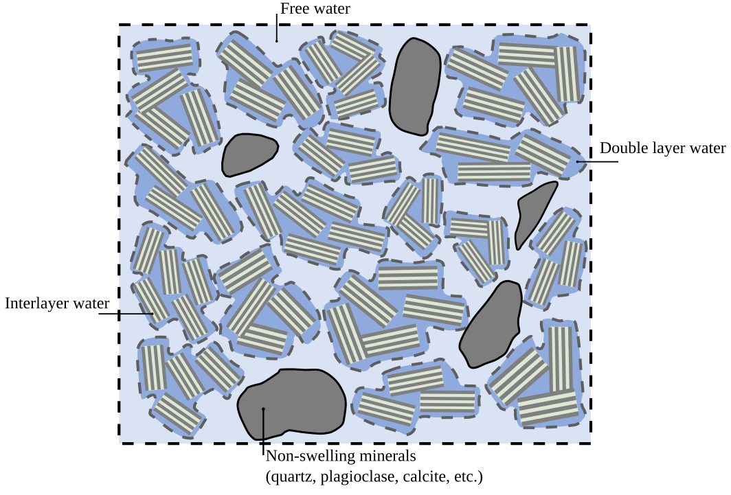
The saddest aspect of this quotation is that it is partly correct: “Scholars have carried out a lot of research” for “decades”, and this view is “generally accepted”.

I cannot say that doing this review has answered my question as to why this is the state of the bentonite research field, but maybe a hint is given by the attitude expressed in TS15 towards modeling and model development. I believe this field will have trouble progressing as long as “modeling” is synonymous with getting arbitrary mathematical descriptions to fit arbitrarily chosen data, padded with empty talk.

Footnotes

[1] As I have commented in the earlier parts: TS15 are fond of using the general terms “clays” and “clay minerals”, while it is clear that the publication mainly focus on systems with substantial ion exchange capacity and swelling properties. Here we will continue to use the term “bentonite” for these systems, and ignore the frequent references in TS15 to more general terms.

[2] Such reinterpretation involves the gradient of the bulk water electrical potential — a potential that TS15 put strictly equal to zero. It also involves the gradient of the Donnan potential — a potential that TS15 mistake for the electric potential in the diffuse layer, when it actually describes the potential difference between bulk and diffuse layer.

[3] Tachi and Yotsuji (2014) report “rock capacity factors” for iodide, which erroneously often are interpreted as anion-accessible porosities. TS15, as we have seen, go “all in” on this concept, while simultaneously admitting that it is fictitious. (?!)

[4] We have noted earlier that it seems very difficult to completely eliminate the effects of interface transfer resistance.

[5] Note that the “correct” value is the arbitrarily selected experimental result 0.42, while the other experimental result of 0.64 is ignored. Also remember that the way this parameter varies with ionic strength is not at all explored by TS15, as they only model results from tests with 0.1 M background concentration.

[6] TS15 report “tortuosities”, rather than actual diffusion coefficients. In a bentonite context, the only way such quantities make sense is as a measure of the diffusion coefficients in terms the corresponding bulk water value, as we discuss here.

[7] I object to that the model parameters are “feasible”. It is in my head a completely ludicrous idea that half the pore volume in pure sodium montmorillonite at 0.8 g/cm3 should contain bulk water — the swelling pressure for a 0.1 M NaCl background concentration is expected to be above 0.4 MPa! Also, the idea that the diffusivity of cesium in montmorillonite is much larger than for sodium, iodide or water is completely unreasonable. In fact, TS15 state that “feasible” simply means a cesium diffusivity that is smaller than for pure bulk water. This shows that they are under the impression that “\(D_e\)”, rather than “\(D_a\)”, quantifies the actual diffusivity in the clay. For a further discussion on this, see here.

[8] Including filter diffusivity in this modeling is certainly not irrelevant per se. However, TS15 merely assign a seemingly random value to this quantity and do nothing more about it. All subsequent inferences are thus contingent on this particular value, yet the authors have neither demonstrated if nor how it influences the overall process.

[9] Although I agree with that these systems don’t contain any appreciable amount of bulk water, we note that no reference is given for this claim. I find this annoying, as TS15 simultaneously don’t hesitate to ascribe 50% bulk water to pure Na-montmorillonite at 0.8 g/cm3. As commented earlier, such a system is expected to have swelling pressure above 0.4 MPa.

[10] We still found serious problems with the model formulation, as further discussed in part 5 of the review.

[11] Also remember that ion exchange is Donnan equilibration!

[12] As always, we should also remember that the distinction betweeen “diffuse layers” and “interlayers” (with quotation marks), or similarly, between “inner” and “outer” basal surfaces, is pure fantasy.

[13] It’s not completely straightforward to extract exact MD values from Tertre et al. (2015). But, discussing them in terms of “surface mobility”, they write: “the mobility for Na is variable from approximately 0.04 to approximately 0.015 when the equivalent fraction of Ca in the solid increases from 0 to 1.” This is a decrease by a factor 2.7.

[14] Note, for instance, that sodium is set to be faster than calcium for the cases of 1.0 M and 0.1 M NaCl, while it is set to be slower than calcium for the cases of 0.05 M and 0.003 M NaCl. Is calcium supposed to be able to retard the sodium flux to such an extent that the sodium ion in the end diffuses slower than the calcium ion?! Note also that the sodium mobility in the TS15 model is lowered by an order of magnitude as the external concentration is only lowered from 0.1 M to 0.05 M! (Or, if the corresponding figure rather than the text is correct, the mobility is even lowered by a factor 40 (the later sections of the paper contain an unacceptable amount of typos of this kind).)

[15] Of course, if ion exchange is supposed to be an “adsorption” process, any cation do “adsorb”. But using such a label for a process that actually may enhance the diffusive flux is, in my opinion, a very bad idea.

[16] To me, the “conceptual framework” promoted in TS15 is “add stuff as you please (but keep bulk water at all costs)”.

[17] Calling the “uphill” effect “anomalous” also seems to contradict the previous general statement that “Diffusion processes through clay materials is the result of a complex interplay of transport and non-linear adsorption processes under the influence of electrostatic fields.”

[18] This only represents a part of “Fig. 1” in Chen et al. (2024), which is explicitly stated to represent compacted water saturated bentonite. I will not elaborate on what is wrong with this figure, but here are some questions to ask: 1. Does this figure represent a realistic size distribution of montmorillonite TOT-layers? 2. Does it represent a typical size distribution of accessory minerals? 3. What is the effective montmorillonite dry density of the depicted system? 4. How is swelling pressure maintained? 5. What keeps “particles” and “aggregates” together? 6. How did this illustration pass peer-review?

Post-publication review: Tournassat and Steefel (2015), part V

This is the fifth part of the review of “Ionic Transport in Nano-Porous Clays with Consideration of Electrostatic Effects” (Tournassat and Steefel (2015) (referred to as TS15 in the following). For background and context please check the first part. Here we make some further comments on electric potentials, and this part is more of an appendix to the previous part, which discussed the proposed model for ion transport in bentonite.1 It is therefore recommended to read up on that part before continuing here.

Even worse problems?

So far in this review we have showed that the model for bentonite proposed in TS15 has both conceptual and mathematical flaws. In the previous part we showed that the “diffuse layer” flux is not derived adequately, although the resulting expression nevertheless can make some sense, if the involved electric potentials are completely reinterpreted. We also noted that the suggested “contributions” to the flux — related to “concentration gradients” (Fickian contribution) and “diffusion potential” (electric field contribution) — make no sense. These “contributions” can, however, be corrected, with the correction term (\(j^\star \)) involving the gradient of \(\Psi^\star\), the electric potential difference between bulk and “diffuse layer”

\begin{equation} j_\mathrm{conc,corr} = j_\mathrm{conc,TS15} + j^\star \end{equation}

\begin{equation} j_\mathrm{E,corr} = j_\mathrm{E,TS15} – j^\star \end{equation}

\begin{equation} j^\star \equiv \frac{A c_\mathrm{bulk} D_\mathrm{DL}zF}{RT} \nabla \Psi^\star \end{equation}

Here \(c_\mathrm{bulk}\) is the bulk water concentration of the considered species (generally a function of the model coordinate \(x\)), \(D_\mathrm{DL}\) is the corresponding diffusion coefficient in the “diffuse layer” domain, \(z\) the charge number, \(F\) the Faraday constant, and \(RT\) the usual thermal energy factor. \(A\) is what TS15 call the “DL enhancement factor”, and is given by (when correctly derived)

\begin{equation} A = e^{-\frac{zF}{RT}\Psi^\star} \end{equation}

The electric potentials in the bulk and “diffuse layer” domain are denoted \(\Psi_\mathrm{bulk}\) and \(\Psi_\mathrm{DL}\), respectively, giving the relation

\begin{equation} \Psi^\star \equiv \Psi_\mathrm{DL} – \Psi_\mathrm{bulk} \tag{1} \end{equation}

With these corrections and reinterpretations it may appear as if the transport model presented in TS15 actually has some merit. Here, however, I would like to point out what I think is a deeper problem, related to the assumption of requiring the various “porosity domains” to be locally in equilibrium. As in the previous part, we focus on the equilibrium between the bulk and “diffuse layer” domains.

In the previous part we did not pay detailed attention to the electric potential difference \(\Psi^\star\). TS15 suggest that \(\Psi^\star\) is to be calculated using the Donnan equilibrium framework. This makes some sense, from the perspective that the model assumes bulk water and “diffuse layer” to be in equilibrium locally, and in the provided examples \(\Psi^\star\) is calculated using the Donnan formula for a 1:1 electrolyte,2

\begin{equation} e^\frac{F\Psi^\star}{RT} = – \frac{q}{2c_\mathrm{bulk}} + \sqrt{\frac{q^2}{4c_\mathrm{bulk}^2} + 1} \end{equation} where \(q\) is a measure of the structural charge in the “diffuse layer”, in the examples set to \(q\) = 0.33 M.

But the requirement of Donnan equilibrium constrains the overall model quite heavily. For example, if we — as in the provided examples — impose concentration profiles in the bulk water, these determine the electric potential profile in this domain, via the Nernst-Planck framework. At the same time, the bulk water concentrations, together with a specified value of \(q\), also completely determine \(\Psi^\star\) (as a function of \(x\)), as well as all “diffuse layer” ion concentrations, via the Donnan equilibrium framework. These “diffuse layer” concentrations will, in turn, determine the electric potential (up to a constant) in this domain, via the Nernst-Planck framework.

But note that the electric potentials in the bulk and “diffuse layer” domains determined in this way, cannot in general also fulfill the requirement for Donnan equilibrium, i.e. \(\Psi^\star \neq \Psi_\mathrm{DL} – \Psi_\mathrm{bulk}\) (cmp. eq. 1). We consequently end up with a contraction, where we have used eq. 1 to determine the “diffuse layer” concentrations, while eq. 1 no longer applies after invoking the Nernst-Planck condition of requiring zero electric current!

This incompatibility is illustrated in the figure above.3 Note that there is nothing special with that the contradiction is here expressed in terms of \(\Psi_\mathrm{bulk}\) and \(\Psi_\mathrm{DL}\) not fulfilling eq. 1. Rather, all of the four relations illustrated in the above figure cannot in general be fulfilled simultaneously. In other words, as far as I see, for an imposed set of concentration profiles in one of the domains, the TS15 model cannot in general simultaneously fulfill these conditions

  • Zero electric current in the bulk water domain
  • Zero electric current in the “diffuse layer” domain
  • Donnan equilibrium between bulk and “diffuse layer”

This flaw is well illustrated in examples 2 and 3 in TS15 (the electric potential is the same for these cases). The electric potential in the bulk water can be calculated from the imposed concentration gradients of the main electrolyte, and is plotted in the figure below (blue line)

Here we have chosen \(\Psi_\mathrm{bulk}(0) = 0\) as reference point. (Note that TS15 are under the false impression that \(\Psi_\mathrm{bulk}(x)\) is zero everywhere.)

In the figure is also plotted the electric potential in the “diffuse layer”, as calculated from the Nernst-Planck framework and the concentration profiles in this domain (orange line; also shown here). As we noted previously, the reason for the much smaller variation of \(\Psi_\mathrm{DL}(x)\) as compared with \(\Psi_\mathrm{bulk}(x)\) is the ever-present counter-ions in the “diffuse layer” domain. Notice further that TS15, in contrast, are under the impression that the electrostatic potential in the “diffuse layer” equals the Donnan potential (red line), while such a profound potential variation is not supposed to affect the electromigration, for unclear reasons.

For \(\Psi_\mathrm{DL}\) we have here chosen the reference point \(\Psi_\mathrm{DL}(0) = \Psi^\star(0)\), i.e. we dictate that the bulk and “diffuse layer” potentials should differ by the Donnan potential when \(x=0\). But this is the only point where this condition is fulfilled: The difference between the electric potentials as calculated in this way (green line) does not at all resemble the Donnan potential!

At the moment, I don’t have the energy to sort out if there is any way out of this paradox, but my guess is that the problem is related to the very different treatments of transport in the \(x\)- and \(y\)-directions in the TS15 model. Remember that the assumption of equilibrium between all domains for a given \(x\)-value is equivalent to assuming infinite mobility in the \(y\)-direction of all species. To me, it appears as the TS15 model attempts to squeeze an intrinsically two-dimensional problem into a one-dimensional form. Note that this problem is not unique for the TS15 model, but arise in any multi-porous, multi-component description which assumes local equilibrium between domains (e.g. Appelo and Wersin (2007)).

Appendix: Comments on Figure 8

Disclaimer: This part functions as an appendix to this already appendix-like part of the review. The reader has been warned.

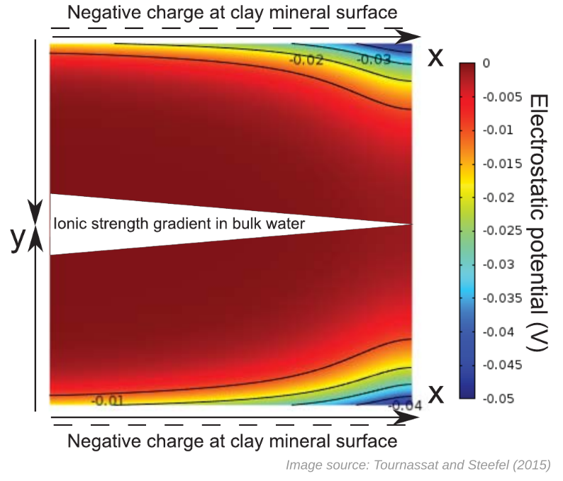
When considering electric potentials in the TS15 model I have developed a need to further comment on “Figure 8”. I alluded to this figure in the previous part of the review when discussing the term “Pseudo 2-D Cartesian system” used by TS15 (a term I don’t understand). “Figure 8” looks like this

The caption reads

Pseudo-2-D Cartesian system with diffusion along the x-axis and electrostatic potential developing along the y-axis due to the negative charge at clay mineral surfaces.

The only reference to this figure in the article text is at the beginning of the section presenting the transport model (Nernst-Planck equation in several “porosity domains”)

In the following, we will consider a pseudo 2-D Cartesian system in which diffusion takes place along the x axis only (Fig. 8).

The more I think about how this figure is included in the article, the more peculiar I find it. The figure clearly shows a quantitative result, as it displays specific values of a two-dimensional electric potential function outside “negative charge at clay mineral surface”. Yet, any real information about this calculation is nowhere to be found, which I see as a major problem (especially as the text is supposed to be a “fully developed text which can be used for self-study, research, or as a text-book for graduate-level courses”). Here we will first discuss information that is not provided, before continuing with speculating about how this figure may have been produced.

Stuff we are not told anything about

The ionic strength

Note that the “ionic strength gradient in bulk water” is only indicated in the figure, but not at all mentioned in the caption or in the text snippet that refers to this figure. Apparently, the physical situation depicted involves “bulk water” where the ionic strength, i.e. the concentration, falls of with the coordinate \(x\). But what is the actual value of this gradient? What are the boundary concentrations? And how has this ionic strength been used when calculating the electrostatic potential? We are not even told what type of electrolyte is considered! Is it 1:1?

Pseudo-2D and length scales

The only two places in TS15 where “Figure 8” is referenced are also the only places where the concept of a “pseudo-2D Cartesian system” is brought up. But what is meant by this term?! To me, it is more than a little strange to base an entire model presentation on a concept that is not really explained.

Taken at face value, the presented figure does not seem to show any “pseudo-“, but a “real” 2D coordinate system. Guided by the variation of the potential in the \(y\)-direction and by the clue that we are outside a negatively charged mineral surface, it’s quite safe to say that we — in the \(y\)-direction — are looking at an actual diffuse layer, as calculated e.g. in the Gouy-Chapman model. The \(y\)-dimension is thus reasonably on the nanometer scale. An ionic strength gradient, however, only makes sense as being on the macroscopic scale. The scale of the \(x\)-dimension is thus reasonably comparable to e.g. that of a laboratory sample, i.e. centimeters or even meters. Although “Figure 8” consequently is oddly scaled (the \(x\)-dimension is at least a million times larger than the \(y\)-dimension), I don’t see any reason to refer to it as “pseudo-2D”. It should of course be completely mandatory to state the length scales when presenting such a figure in a peer-reviewed scientific journal.

Further, we note that the figure seems to depict two copies facing each other of the same potential function, with one copy being flipped vertically (this explains the two oppositely pointing \(y\)-axes). Is this the reason for calling the coordinate system “Pseudo-2D”? But this manipulation (two copies facing each other) seems only to be for illustrative purposes, and has no impact on what actually seems to have been calculated.4

Surface charge

The potential is supposed to be “developing […] due to the negative charge at the clay mineral surfaces”. But then a surface charge density must have been specified when calculating the potential. Needless to say, this value should have been stated.

Stuff that is incorrect or odd

“Developing” potential

The figure caption “explains” that an electrostatic potential “develop[s] along the \(y\)-axis”. But what is significant is that an electric field is present near the surface. And, as we have brought up earlier, an electric field is equivalent to a potential variation. To put focus on that a potential “develops”, rather than that the potential varies, mostly misses the point. Also, why is the word “develop” used here? It suggests some sort of ongoing (unexplained) process.

“Developing” potential along the y-axis

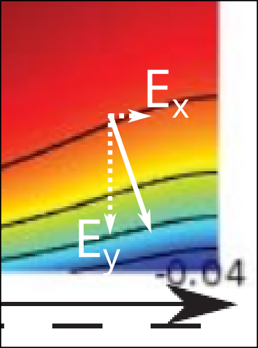
A clear illustration that something is missed when speaking of potentials rather than fields is that TS15 implies that this “development” occurs exclusively in the \(y\)-direction. Note that an electric field is directed normal to the lines of constant electric potential. It is thus completely clear from the figure itself that the electric field is not in general directed solely in the \(y\)-direction!

This type of manifestation of an electric field in the \(x\)-direction relates to the complications discussed earlier of having a Donnan potential that varies with \(x\).

The potential has not resulted from solving the Nernst-Planck equation

Even though the purpose of the section is a treatment of the Nernst-Planck framework for transport of ionic charges, “Figure 8” does not present the result of a Nernst-Planck calculation. A main objective of such a treatment is to calculate the gradient of the electric potential (in the \(x\)-direction), i.e. an electric field. In contrast, the figure clearly shows that the potential is essentially zero, some distance away from the surface.

We note that a zero electric potential in the region that the authors presumably classify as “bulk” (some nanometers away from the surface…) is in line with the erroneous procedure of setting the bulk electric potential identically zero in the derivation of the Nernst-Planck flux.

What I think is illustrated/has been calculated

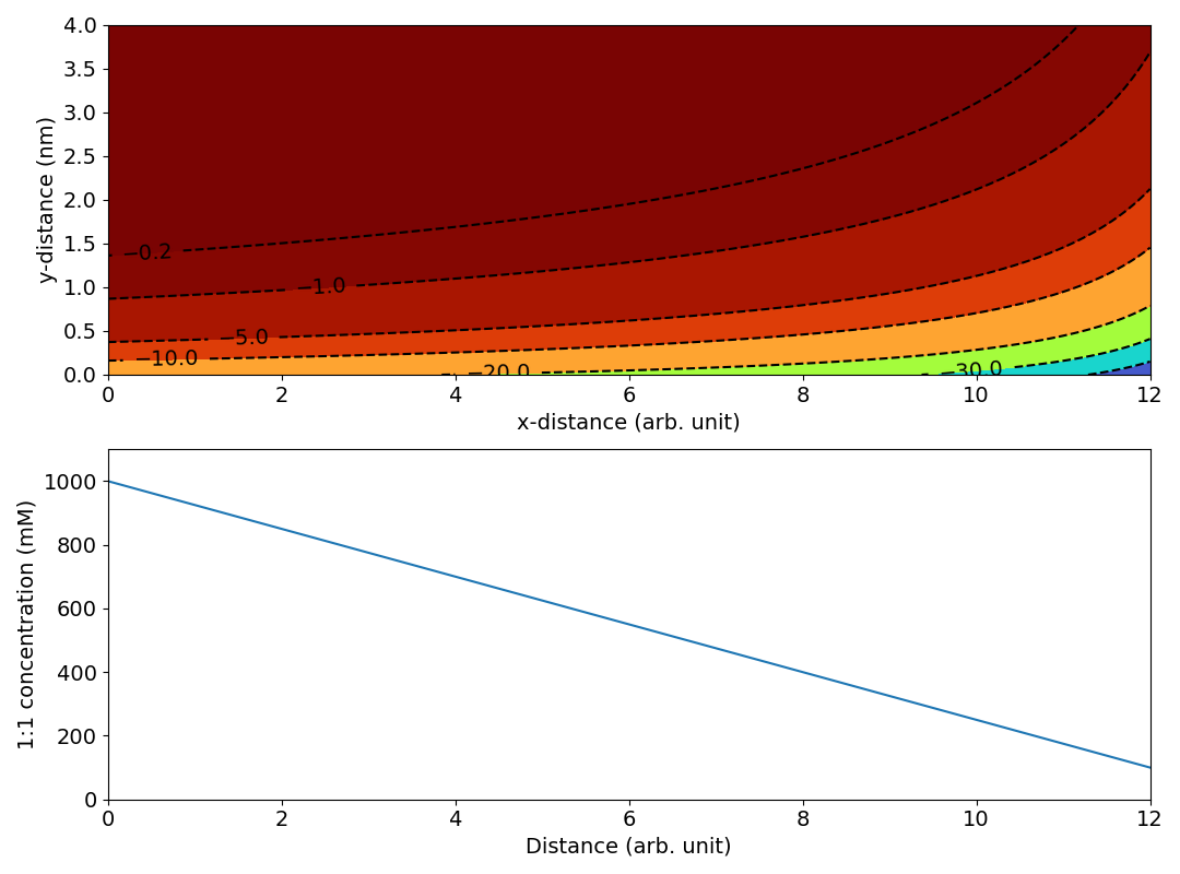
My guess is that “Figure 8” has been produced by calculating a set of potential profiles (in the \(y\)-direction) from the Gouy-Chapaman model for a given set of values of the ionic strength. These profiles have then simply been “stacked” in the \(x\)-direction. Below are some attempts to recreate “Figure 8” using this approach.

Since no parameters are given in TS15, we have to make several assumptions. For the figure below is assumed a linear profile of a 1:1 electrolyte that falls from 1000 mM at \(x=0\) to 100 mM at \(x=12\). We furthermore assume a surface charge density of 0.04 C/m2.

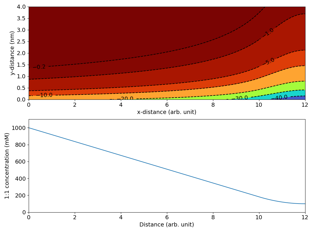
The magnitude and variation of this potential is comparable to that in “Figure 8” (the unit for the electric potential is here mV). We may note, however, that the linear ionic strength profile results in lines of constant electric potential that more and more “bends away” from the surface. This is because the Debye length in a 1:1 electrolyte depends on ionic strength as \(1/\sqrt{I}\). In contrast, the lines of constant potential in “Figure 8” are seen to “bend back”, suggesting a leveling off of the ionic strength, like this

If the present speculations are correct, why on earth has such a concentration profile been chosen? More broadly, why is this type of figure at all presented? If the authors simply want to show the quantities being calculated, why not provide a schematic illustration rather than a quantitative calculation? And if they want to present an actual calculation — which for unclear reasons does not involve the Nernst-Planck framework — they must of course provide a reader with enough information to make it understandable.

Update (260824): Part VI of this review is found here.

Footnotes

[1] As I have commented in the earlier parts: TS15 are fond of using the general terms “clays” and “clay minerals”, while it is clear that the publication mainly focus on systems with substantial ion exchange capacity and swelling properties. Here we will continue to use the term “bentonite” for these systems, and ignore the frequent references in TS15 to more general terms.

[2] TS15 are under the impression that \(\Psi_\mathrm{bulk}= 0\), and they believe that they calculate \(\Psi_\mathrm{DL}\) rather than \(\Psi^\star\). They furthermore emphasize that a more accurate calculation involves integrating the Poisson-Boltzmann equation (and claim falsely that the Donnan equilibrium “model” is based on an approximation of the Poisson-Boltzmann equation). But under all circumstances, the TS15 model requires specifying an arbitrary size of the “diffuse layer”; in the examples is used a width of 3 nm, which approximately corresponds to 3, 1 and 0.3 Debye lengths, respectively, for 1:1 background concentrations 0.1 M, 0.01 M, and 0.001 M. As we have discussed in the blog post on why multi-porosity models cannot be taken seriously, such a partitioning requires that a mechanism is provided for how equilibrium is maintained (i.e. why the “diffuse layer” does not occupy the full pore volume). TS15 do not supply such a mechanism, and neither does any other author promoting multi-porous models.

[3] In this figure, \( \left \{ c_{\mathrm{bulk} ,i} \right \} \) denotes the complete set of imposed concentrations in the bulk water domain. The corresponding set of species concentrations in the “diffuse layer” is denoted \(\left \{ c_{\mathrm{DL},i}\right \}\).

[4] Even if this choice is only “cosmetic”, I actually don’t understand why the figure is presented like this. Is it supposed to depict an (insanely long) interlayer? Perhaps with a “bulk water” phase squeezed in the middle? The same authors have actually presented such types of figures in later publications. As I discuss here, such a representation of a “bulk water” phase is nonsense.

Post-publication review: Tournassat and Steefel (2015), part IV

This is the fourth part of the review of “Ionic Transport in Nano-Porous Clays with Consideration of Electrostatic Effects” (Tournassat and Steefel, 2015) (referred to as TS15 in the following). For background and context please check the first part. This part covers the two sections “Constitutive equations for diffusion in bulk, diffuse layer, and interlayer water” and “Relative contributions of concentration, activity coefficient and diffusion potential gradients to total flux”.

“Constitutive equations for diffusion in bulk, diffuse layer, and interlayer water”

This section presents a mathematical formulation of ion diffusion in bentonite,1 based on the material descriptions in the earlier sections. As we have previously noted, these descriptions are fundamentally flawed in several respects. In particular, compacted bentonite is presented as consisting of stacks (called “particles”), where it is supposed to make sense to differ between external and internal interface water. TS15 also mean that compacted bentonite (sometimes?) is supposed to contain a bulk water phase.

As I have commented on in earlier parts, the only reason I can see to provide this nonsensical material description is as an attempt to to motivate a macroscopic, multi-porous model of bentonite. Here, TS15 make this claim quite explicit, as they write

Still it is possible to define three porosity domains, or water domains, that can be handled separately: the bulk water, the diffuse layer water and the interlayer water, the properties for which can be each defined independently.

This is in essence what I have referred to as “the mainstream view” of bentonite. It is basically “possible” to define anything, but the real question is if provided definitions are relevant and useful. And, as we have already discussed in detail, there is no rationale for introducing these “porosity domains” when modeling water saturated, compacted bentonite.2

Here we will first comment on the conceptual aspects of the provided mathematical description. Thereafter, we will delve into the mathematical formulations, as I’m quite convinced that these are not correct. Unfortunately, this latter part will be quite burdened with equations and notation, but for the motivated reader I think it may be worth going through.

Conceptual aspects

TS15 choose the Nernst-Planck description of ion diffusion, and begin by commenting that this is more rigorous than using Fick’s law. I certainly agree with that a general description of ion diffusion in bentonite requires treating electrostatic couplings between the various system components (TOT-layers, ions). I don’t think, however, that putting up a massively complex description of multi-component diffusion in “three porosity domains” is the appropriate starting point for including such couplings. Since we have every reason to believe that e.g. no bulk water phase is present, I mean that this type of treatment only leads us astray from understanding the actual processes involved (we will return to this aspect in later parts of the review).

Also, as the “Fickian” aspect was the focus of the earlier section on diffusion, a reader of TS15 could here understandably get the impression that a Nernst-Planck treatment will “fix” the “issues” addressed there. But, as we have already discussed in some detail, the shortcomings of the traditional sorption-diffusion model are not solved by including multi-component diffusion in a bulk water phase. They are solved by removing the bulk water phase.

Although the above quotation states that the various “porosity domains” can be handled separately, and that their properties can be defined independently, this is not what is done in TS15. Rather, the treatment of any “porosity domain” assumes equilibrium with the corresponding bulk water phase. The entire description in TS15 is thus fully centered around the bulk water phase.

TS15 insist on treating their model quantities as functions of two spatial coordinates (\(x\) and \(y\)), in what they refer to as a “pseudo 2-D Cartesian system” (I don’t fully understand what that means). Diffusive flux is only assumed to take place in the \(x\)-direction, while the “\(y\)”-dimension is used for stacking the different “porosity domains”. The description can be schematically illustrated like this

Here we have for illustrative purposes discretized the various components in \(x\)- and \(y\)-directions. The bulk water domain is colored blue, the “interlayer” domain pink, and the “diffuse layer” domain green. For a given \(x\)-position, the “diffuse layer” and the “interlayer” domains are assumed to always be in equilibrium with the corresponding bulk water phase. TS15 nowhere consider the length scale in the \(y\)-direction (is it therefore the coordinate system is referred to as “pseudo 2-D”?), which in practice makes the model a collection of 1-dimensional domains that are in equilibrium locally. Note that even though diffusion only is accounted for in the \(x\)-direction, transport occurs also in the \(y\)-direction, as a consequence of equilibration between the “porosity domains”.

This description is exactly what we have investigated in the blog post on why multi-porous models cannot be taken seriously. To summarize what was said there, without properly defining the length scales, it makes no sense to “short-cut” the model in the \(y\)-direction (to assume equilibrium for all domains at the same \(x\) is in a sense equivalent to assuming infinitely high mobility of all components in the \(y\)-direction). And even if we assume that such an assumption is valid — which would mean that we consider a thin strip of stacked parallel domains, where the extension in \(y\) is negligible in comparison to the extension in \(x\) — the resulting model has really nothing to do with actual bentonite. As we concluded in the multi-porosity blog post, the only way to make sense of this type of description is as a set of macroscopic continua that are assumed to be locally in equilibrium. How this equilibrium is supposed to be maintained has never been suggested by any proponent of this description. Note that this description (in particular the existence of a bulk water phase in equilibrium) disqualifies the model for describing swelling and swelling pressure.

Incorrect application of the Nernst-Planck framework

While the presented model makes little sense conceptually, TS15 also fail in applying the Nernst-Planck framework. The problem arises, as far as I can see, from that they don’t fully recognize the role of the electric potential.

As we now begin scrutinizing the details of the formulation, we will suppress the variables \(x\) and \(y\) in order to, hopefully, make the equations a little more readable. It should be understood that any quantity is evaluated for some specific value of \(x\), and that all “porosity domains” are supposed to be in equilibrium at the same value of \(x\).

The electro-chemical potential

In most standard thermodynamic text books we learn that the chemical potential governs the equilibrium associated with mass transfer. Just as e.g. pressure and temperature (which govern mechanical and thermal equilibrium, respectively), the chemical potential is defined by a specific derivative of a thermodynamic potential, e.g.3

\begin{equation} \bar{\mu} = \left ( \frac{\partial G}{\partial n} \right )_{T,p} \tag{1} \end{equation}

where \(G\) is the Gibbs free energy, \(n\) number of moles, \(p\) pressure, and \(T\) temperature. The corresponding mass flux is generally written

\begin{equation} j = -\frac{cD}{RT}\nabla \bar{\mu} \tag{2} \end{equation}

where \(c\) is concentration, \(D\) the diffusion coefficient4, and \(RT\) the usual absolute temperature factor. Here, and in the following, we use the symbol \(\nabla\), which denotes the general gradient operator, but since the model is effectively one-dimensional, it can simply be seen as a neat way of writing \(\partial/\partial x\).

For charged species, it is common to refer to the quantity defined in eq. 1 as the electro-chemical potential, and write it as composed of an “ordinary” and a purely “electrical” part

\begin{equation} \bar{\mu} = \mu + zF\Psi \tag{3} \end{equation}

where \(z\) is the charge number of the considered species, \(F\) is the Faraday constant and \(\Psi\) is the electric potential. The “ordinary” chemical potential \(\mu\) (without bar) is, perhaps a bit confusingly, also often referred to as the chemical potential. I will here continue to refer to this part as “ordinary”. The “ordinary” chemical potential is furthermore conventionally expressed in terms of a reference potential (\(\mu^0\)) and an activity \(a\)

\begin{equation} \mu = \mu^0 + RT\ln a \tag{4} \end{equation}

A lot can be said about the decomposition in eq. 3, but it is clear that singling out an electric potential term is useful in e.g. electrochemistry or for describing charged clay. It should, however, be kept in mind that mass transfer is fundamentally governed by gradients in \(\bar{\mu}\); always keeping eqs. 1 and 2 in mind will avoid us from making mistakes, because the mass transfer rate relates to the “total” (i.e. electrochemical) potential, and for charge neutral species the description reduces to gradients in the “ordinary” chemical potential.

Nernst-Planck flux

Combining eqs. 3 and 4 gives

\begin{equation} \bar{\mu} = \mu^0+RT \ln a + zF\Psi \tag{5} \end{equation}

with the corresponding flux (eq. 2)

\begin{equation} j = -cD\nabla \ln a -\frac{cDzF}{RT} \nabla \Psi \end{equation}

Expressing the activity in terms of an activity coefficient, \(a = \gamma c\), the flux can also be written (TS15 are quite fond of including activity coefficients explicitly)

\begin{equation} j = -D\nabla c -cD\nabla \ln \gamma -\frac{cDzF}{RT} \nabla \Psi \tag{6} \end{equation}

Considering an arbitrary set of diffusing charged species (using the index \(i\)), and utilizing that the electric current is zero, lead to an expression for the electric potential gradient

\begin{equation} \nabla \Psi = -\frac{RT}{F}\frac{\sum z_iD_i \left ( \nabla c_i + c_i \nabla \ln \gamma_i \right )}{\sum z_i^2 D_i c_i} \tag{7} \end{equation}

Misunderstanding the electric potential

For the bulk water phase, TS15 indeed provide an expression for the flux that is essentially the same as eq. 6 (their eq. 37), and which they refer to as the Nernst-Planck equation. They claim, however, that the electrochemical potential in this case lack an electric potential term (my emphasis)5,6

In absence of an external electric potential, the electrochemical potential in the bulk water can be expressed as (Ben-Yaakov 1981; Lasaga 1981) \begin{equation} \bar{\mu}_\mathrm{bulk} = \mu^0+RT \ln a_\mathrm{bulk} \end{equation}

But even without an externally applied electric field,7 a zero bulk electric potential cannot be assumed, of course, if the goal is to treat individual ion mobilities; as just shown, the gradient in electric potential that appears in eq. 6 is a result of a corresponding term in the electrochemical potential (eq. 5). Oddly, TS15 seem to treat the electric potential term in the flux as a quantity unrelated to the electrochemical potential, giving it a separate symbol, \(^\mathrm{b}\Psi_\mathrm{diff}\), and writing

\(^\mathrm{b}\Psi_\mathrm{diff}\) is the diffusion potential that arises because of the diffusion of charged species at different rates.

It may be natural for a reader at this point to simply assume that TS15 have missed writing out the term \(zF^\mathrm{b}\Psi_\mathrm{diff}\) when stating the electrochemical potential. But this seems to be a genuine misunderstanding rather than a mistake/typo, because the pattern repeats in the derivation of the flux in the other “porosity domains”.

For e.g. the “diffuse layer”,8 TS15 recognize the presence of an electric potential in the expression for the electrochemical potential, writing it (this is more awkwardly expressed in eq. 42 in TS15)

\begin{equation} \bar{\mu}_\mathrm{DL} = \mu^0 + RT\ln a_\mathrm{DL} + zF\Psi_\mathrm{DL} \tag{8} \end{equation}

where index “DL” refers to quantities in the “diffuse layer”.

However, the corresponding flux expression contains a different potential, labelled \(^\mathrm{DL}\Psi_\mathrm{diff}\) (eq. 46 in TS15)

\begin{equation} j_\mathrm{DL} = -\frac{c_\mathrm{DL}D_\mathrm{DL}}{RT}\nabla \bar{\mu}_\mathrm{DL} -\frac{c_\mathrm{DL}D_\mathrm{DL}zF}{RT} \nabla ^{\mathrm{DL}}\Psi_\mathrm{diff} \tag{9} \end{equation}

TS15 don’t further comment what \(^{\mathrm{DL}}\Psi_\mathrm{diff}\) is supposed to represent, but it must reasonably be understood as “the diffusion potential that arises because of the diffusion of charged species at different rates”, in analogy with what was claimed for the bulk water phase. Note that when eq. 8 is combined with eq. 9, the flux expression contains two different electric potential gradients! (TS15 never address this oddity.)

It is thus quite clear that TS15 misunderstand the function of the electric potential in the Nernst-Planck framework. When presenting the expression for the “diffuse layer” flux (eq. 9), they also refer to Appelo and Wersin (2007), who, in turn, express the misconception explicitly9

The gradient of the electrical potential [in the expression for the flux] originates from different transport velocities of ions, which creates charge and an associated potential. This electrical potential may differ from the one used in [the expression for the electro-chemical potential], which comes from a charged surface and is fixed, without inducing electrical current.

I cannot understand this passage in any other way than that Appelo and Wersin (2007) are under the impression that different electric potentials can simultaneously act independently in a given point. And it seems like TS15 are under some similar impression.

This ignorance leads to more errors in the description of the “diffuse layer” in TS15. We should remember that the promoted model requires the “diffuse layer” and bulk water domains to be in equilibrium (for the same coordinate value \(x\)). When TS15 express this condition, i.e. \(\bar{\mu}_\mathrm{DL} = \bar{\mu}_\mathrm{bulk}\), they again leave out the electric potential in the bulk water (eq. 42 in TS 15)

\begin{equation} \mu^0 + RT\ln a_\mathrm{DL} + zF\Psi_\mathrm{DL} = \mu^0 + RT\ln a_\mathrm{bulk}\;\:\;\;\;\;\;\mathrm{(WRONG)} \tag{10} \end{equation}

eq. 10 can be rewritten

\begin{equation} a_\mathrm{DL} = a_\mathrm{bulk}\cdot e^{-\frac{zF}{RT}\Psi_\mathrm{DL}} \;\:\;\;\;\;\;\mathrm{(WRONG)} \tag{11} \end{equation}

TS15 utilize a simplified version of eq. 11, expressed in terms of concentrations rather than activities, by assuming identical activity coefficients in the two domains10

\begin{equation} c_\mathrm{DL} = c_\mathrm{bulk}\cdot e^{-\frac{zF}{RT}\Psi_\mathrm{DL}} \;\:\;\;\;\;\;\mathrm{(WRONG)} \tag{12} \end{equation}

Note that the exponential in eqs. 11 and 12 actually should contain the electric potential difference between “diffuse layer” and bulk (see below).

As TS15 have not included any electric potential in the bulk water phase, they continue by incorrectly substituting \(RT\nabla \ln a_\mathrm{bulk}\) for \(\nabla\bar{\mu}_\mathrm{DL}\) in eq. 9 (i.e. they use the incorrect relation in eq. 10), giving (TS15 eq. 47)

\begin{equation} j_\mathrm{DL} = -c_\mathrm{DL}D_\mathrm{DL}\nabla \ln a_\mathrm{bulk} -\frac{c_\mathrm{DL}D_\mathrm{DL}zF}{RT} \nabla ^{\mathrm{DL}}\Psi_\mathrm{diff} \;\;\;\;\mathrm{(WRONG)} \tag{13} \end{equation}

Note that this additional error “solves” the earlier pointed out problem of having two electric potential gradients.

By utilizing the requirement of zero electric current, eq. 13 gives

\begin{equation} \nabla ^{\mathrm{DL}}\Psi_\mathrm{diff} = -\frac{RT}{F}\frac{\sum z_iD_{\mathrm{DL},i}c_{\mathrm{DL},i} \nabla \ln a_{\mathrm{bulk},i} }{\sum z_i^2 D_{\mathrm{DL},i} c_{\mathrm{DL},i}} \;\:\;\;\;\;\;\mathrm{(WRONG)} \tag{14} \end{equation}

By substituting eq. 12 into this expression, we end up with the formula for the gradient of the mysterious potential \(^{\mathrm{DL}}\Psi_\mathrm{diff}\) (TS15 eq. 48)

\begin{equation} \nabla ^{\mathrm{DL}}\Psi_\mathrm{diff} = \end{equation} \begin{equation} -\frac{RT}{F}\frac{\sum z_iD_{\mathrm{DL},i} e^{-\frac{zF}{RT}\Psi_\mathrm{DL}} \left ( \nabla c_{\mathrm{bulk},i} + c_{\mathrm{bulk},i}\nabla \ln \gamma_{\mathrm{bulk},i} \right )} {\sum z_i^2 D_{\mathrm{DL},i} e^{-\frac{zF}{RT}\Psi_\mathrm{DL}}c_{\mathrm{bulk},i}} \;\mathrm{(WRONG)} \tag{15} \end{equation}

At face value, eq. 15 is a quite weirdly looking equation, as it relates two electric potentials — \(^{\mathrm{DL}}\Psi_\mathrm{diff}\) and \(\Psi_\mathrm{DL}\) — that both are supposed to be associated with the “diffuse layer”. But, as we will see below, there is actually a way to make some sense of eq. 15, by completely reinterpreting what these potentials represent.

A “correct” formulation

Update (260803): The electrostatic potential within the homogeneous mixture model is treated here.

Most of the errors pointed out above are corrected by including the electric potential in the bulk water and writing the condition for equilibrium as (compare eq. 10)

\begin{equation} \mu^0 + RT\ln a_\mathrm{DL} + zF\Psi_\mathrm{DL} = \mu^0 + RT\ln a_\mathrm{bulk} + zF\Psi_\mathrm{bulk} \tag{16} \end{equation}

Writing the electric potential difference between “diffuse layer” and bulk water as11

\begin{equation} \Psi^\star \equiv \Psi_\mathrm{DL} – \Psi_\mathrm{bulk} \tag{17} \end{equation}

eq. 16 can be rewritten

\begin{equation} a_\mathrm{DL} = a_\mathrm{bulk}\cdot e^{-\frac{zF}{RT}\Psi^\star} \tag{18} \end{equation}

Note that, when correctly derived, eq. 18 naturally contains the difference in electric potential between “diffuse layer” and bulk.

The flux in the “diffuse layer” is (eq. 6)

\begin{equation} j_\mathrm{DL} = -c_\mathrm{DL} D_\mathrm{DL} \nabla \ln a_\mathrm{DL} – \frac{c_\mathrm{DL} D_\mathrm{DL} zF}{RT} \nabla \Psi_\mathrm{DL} \tag{19} \end{equation}

But if we now plug in eq. 18 in eq. 19 we of course get

\begin{equation} j_\mathrm{DL} = -c_\mathrm{DL} D_\mathrm{DL} \nabla \ln a_\mathrm{bulk} + \frac{c_\mathrm{DL} D_\mathrm{DL} zF}{RT} \nabla \Psi^\star – \frac{c_\mathrm{DL} D_\mathrm{DL} zF}{RT} \nabla \Psi_\mathrm{DL}, \end{equation} which can be simplified to \begin{equation} j_\mathrm{DL} = -c_\mathrm{DL} D_\mathrm{DL} \nabla \ln a_\mathrm{bulk} – \frac{c_\mathrm{DL} D_\mathrm{DL} Fz}{RT} \nabla \Psi_\mathrm{bulk}, \tag{20} \end{equation} and, by identifying the electro-chemical potential in the bulk \begin{equation} j_\mathrm{DL} = -\frac{c_\mathrm{DL} D_\mathrm{DL}}{RT} \left ( RT \nabla \ln a_\mathrm{bulk} + Fz \nabla \Psi_\mathrm{bulk} \right ) = -\frac{c_\mathrm{DL} D_\mathrm{DL}}{RT} \nabla \bar{\mu}_\mathrm{bulk} \end{equation}

This whole “derivation” leads back to the rather trivial result that the flux in the diffuse layer is given by eq. 2, which we could have written down from the start! (because the model assumes \(\bar{\mu}_\mathrm{bulk} = \bar{\mu}_\mathrm{DL}\); eq. 16)

As TS15 have established the expression for the gradient of the electrochemical potential in the bulk water phase (which is implicit in their eq. 40), there should strictly be no need to consider a new expression for the same quantity in any other phase. Rather, they could simply have used the bulk water expression in all “porosity domains”, as a consequence of the assumption that these are all supposed to be in equilibrium. In a sense, this is actually what is done in TS15 — mainly by chance! — by establishing eq. 13 (their eq. 47).

Comparing with eq. 20, we see that the incorrect eq. 13 can be “saved” by reinterpreting \(^{\mathrm{DL}}\Psi_\mathrm{diff}\) as \(\Psi_\mathrm{bulk}\). Similarly, as TS15 assume the bulk electric potential to be zero, eq. 15 can be “saved” by also reinterpreting \(\Psi_\mathrm{DL}\) as \(\Psi^\star\) in that expression.12 I find this quite hilarious: By making several errors in its derivation, eq. 15 is in a sense a correct expression for the electric potential gradient in the bulk water — a potential that TS15 has put identically equal to zero.

But even if the total flux in the “diffuse layer” is correctly given by combining eqs. 12, 13 and 15 (and by completely ignoring what TS15 mean \(\Psi_\mathrm{DL}\) and \(^{\mathrm{DL}}\Psi_\mathrm{diff}\) represent), TS15 continue by defining the separate terms in eq. 13 as contributions from the “concentration gradient”, and the “diffusion potential”. As we will explore next, this interpretation fails miserably.

“Relative contributions of concentration, activity coefficient and diffusion potential gradients to total flux”

According to TS15, the “concentration gradient” and the “diffusion potential” contributions to the “diffuse layer” flux are given by, respectively (TS15 eq. 50 and below)

\begin{equation} j_\mathrm{conc,TS15} = -D_\mathrm{DL}A\nabla c_\mathrm{bulk} \tag{21} \end{equation}

and

\begin{equation} j_\mathrm{E,TS15} = zD_\mathrm{DL}c_\mathrm{bulk}A\frac{\sum z_iD_{\mathrm{DL},i}A_i\left ( \nabla c_{\mathrm{bulk},i} + c_{\mathrm{bulk},i} \nabla \ln \gamma_{\mathrm{bulk},i} \right )} {\sum z_i^2 D_{\mathrm{DL},i} A_i c_{\mathrm{bulk},i}} \tag{22} \end{equation}

Here we use the index “conc” for the “concentration gradient” contribution, and “E” for the “diffusion potential” contribution. \(A\) is referred to as a “DL enrichment factor”, and is essentially defined as the concentration ratio \(c_\mathrm{DL}/c_\mathrm{bulk}\). Using the incorrect relation in eq. 12, TS15 write these as \(A = e^{-\frac{zF}{RT}\Psi_\mathrm{DL}}\), but, as we see from eq. 18, they are really given by13 (we continue assuming identical activity coefficients in the two domains)

\begin{equation} A = e^{-\frac{zF}{RT}\Psi^\star} \tag{23} \end{equation}

TS15 also define a third contribution, related to the gradient of the bulk water activity coefficient. Here we will not further discuss this contribution, as it does not give any additional insight. Moreover, since TS15 anyway derive their model under the unjustified assumption that activity coefficients in the “diffuse layer” and the bulk water are identical, I cannot see the use of including their spatial variation in the description.14 (TS15 spend a couple of pages on activity coefficient models that we will ignore.)

Examples

To explore the various couplings in the presented model, TS15 apply the Nernst-Planck framework in three examples. We can see immediately from the presented graphs that their partitioning of the total flux in “concentration gradient” and “diffusion potential” contributions makes no sense.

“Example 2” imposes constant concentration gradients in the bulk water of NaCl and corresponding \(^{22}\mathrm{Na}^+\) and \(^{36}\mathrm{Cl}^-\) tracers; the NaCl concentration drops from 0.1 M to 0.001 M, and the tracer concentrations drop from 10-9 M to 10-11 M (domain length is 10 mm).

The corresponding sodium and chloride tracer concentrations in the “diffuse layer” look like this15

These profiles make sense: bulk water ionic strength decreases with distance, but so do the tracer concentrations. For the process of accumulating \(^{22}\mathrm{Na}^+\) in the diffuse layer, these two effects oppose each other, resulting in a quite flat profile. We thus expect the corresponding “concentration gradient” contribution to the flux to be quite moderate, and to fall off with distance (as the profile flattens with distances). The corresponding flux graph presented in TS15, however, looks completely different16

This plot makes no sense: The “concentration gradient” contribution is seen to increase quite dramatically with distance, rather than falling off. The value of this contribution is also orders of magnitude too large, given the imposed sodium diffusion coefficient of 1.33⋅10-10 m2/s. Moreover, the “concentration gradient” contribution is “compensated” by an equally nonsensical “diffusion potential” contribution. Note, for instance, that the “diffusion potential” contribution is negative, which implies that the corresponding electric field is supposed to be directed towards higher concentrations. This can certainly not be the case, as the electric potential gradient is caused by the negative ion having higher mobility than the positive ion (chloride diffusivity is set to 2.03⋅10-10 m2/s).

In “example 3”, the tracer concentrations in the bulk is set to a constant value (1⋅10-9 M), while the same concentration gradient as in “example 2” is maintained for the main NaCl electrolyte (from 0.1 M to 0.001 M). We thereby expect the corresponding \(^{22}\mathrm{Na}^+\) concentration in the “diffuse layer” to strongly increase with distance, which is also what is presented in TS15

while the corresponding flux plot looks like this16

This plot is almost comically absurd. According to TS15, the highly skewed concentration profile above is supposed to give no (zero, nil, 0) contribution to the flux (we see from eq. 21 that this is a consequence of that this “contribution” is directly proportional to the concentration gradient in the bulk). Instead, the huge flux is supposed to be caused entirely by an electric field that has the wrong direction! I can’t even really begin to imagine how these two plots have ended up next to each other in a peer-reviewed published article.

Note that the flux associated with a concentration gradient is what we may reasonably call a “Fickian” contribution. If TS15 mean (and they do) that these examples demonstrate how ion diffusion in bentonite works, we can understand the focus on the “Fickian” aspect at the beginning of the article (covered here). But the only reasonable response to these outlandish results is that they demonstrate that the definitions of eqs. 21 and 22 simply make no sense.

The real concentration gradient and electric field contributions

The only reasonable way to define “concentration gradient” and “diffusion potential” contributions to the “diffuse layer” flux is as the two terms in eq. 19, respectively. To rewrite these, we utilize eq. 16 (or 18), giving for the “concentration gradient” contribution (we continue ignoring activity coefficients)

\begin{equation} j_\mathrm{conc, corr} = -c_\mathrm{DL} D_\mathrm{DL} \nabla \ln c_\mathrm{DL} = \end{equation} \begin{equation} -c_\mathrm{DL} D_\mathrm{DL} \nabla \ln c_\mathrm{bulk} + \frac{c_\mathrm{DL} D_\mathrm{DL}zF}{RT} \nabla \Psi^\star = \end{equation} \begin{equation} -D_\mathrm{DL} A \nabla c_\mathrm{bulk} + \frac{A c_\mathrm{bulk} D_\mathrm{DL}zF}{RT} \nabla \Psi^\star = j_\mathrm{conc, TS15} + j^\star \tag{24} \end{equation}

where we have defined

\begin{equation} j^\star \equiv \frac{A c_\mathrm{bulk} D_\mathrm{DL}zF}{RT} \nabla \Psi^\star. \tag{25} \end{equation}

In the same manner, the correct “diffusion potential” contribution is

\begin{equation} j_\mathrm{E, corr} = – \frac{c_\mathrm{DL} D_\mathrm{DL} zF}{RT} \nabla \Psi_\mathrm{DL} = \end{equation} \begin{equation} – \frac{D_\mathrm{DL}Ac_\mathrm{bulk} zF}{RT} \nabla \Psi_\mathrm{bulk} – \frac{D_\mathrm{DL}Ac_\mathrm{bulk} zF}{RT} \nabla \Psi^\star = \end{equation} \begin{equation} D_\mathrm{DL}Ac_\mathrm{bulk} z \frac{\sum z_iD_iA_i\left ( \nabla c_{\mathrm{bulk},i} + \nabla c_{\mathrm{bulk},i} \ln \gamma_{\mathrm{bulk},i} \right )} {\sum z_i^2 D_i A_i c_{\mathrm{bulk},i}} – \frac{D_\mathrm{DL}Ac_\mathrm{bulk} zF}{RT} \nabla \Psi^\star = \end{equation} \begin{equation} j_\mathrm{E, TS15} – j^\star \tag{26} \end{equation}

where we have utilized that \(\nabla \Psi_\mathrm{bulk}\) is actually what is expressed in eq. 15 (where \(\Psi_\mathrm{DL}\) should be replaced by \(\Psi^\star\)).

We note that, to compensate the nonsensical expressions given in TS15, we should add the term \(j^\star\) (eq. 25) to the “concentration concentration” contribution (eq. 21), and subtract the same term from the “diffusion potential” contribution (eq. 22). Making these corrections gives the following components of the tracer fluxes in “example 2”

This is an infinitely more reasonable situation than what is depicted in TS15. Although the sodium flux has a non-negligible contribution from the electric field, the larger contribution is still from the concentration gradient (and none of these are gigantic terms that cancel). The concentration contribution also falls off with distance, in accordance with the shape of the concentration profile.

For chloride, the field contribution to the flux is negligible, i.e. this flux is essentially fully governed by the concentration gradient. The electric field contributions for both ions are also seen to have the correct signs: the electric field is directed from high to low concentration, and mainly functions to boost the sodium transport, in order to “keep up” with the faster chloride ions.

For “example 3” we get the following picture

The corrected \(^{22}\mathrm{Na}^+\) flux is essentially fully due to the concentration gradient, in absolute contrast to what is concluded in TS15, who mean that this flux is completely governed by an electric field in the wrong direction. Also the \(^{36}\mathrm{Cl}^-\) transport is basically solely governed by the concentration gradient, rather than by an incorrectly directed electric field (as stated in TS15). In conclusion, most of the “diffuse layer” diffusion in these examples can actually be classified as “Fickian”.

We may also investigate the electric potential profile in the “diffuse layer” in both of these examples (this is the same in the two cases, as the main electrolyte distribution does not change)

Here we have chosen the reference \(\Psi_\mathrm{DL}(0) = 0\). The total potential drop is only about 1 mV. Such a relatively small drop is reasonable because the denominator in the Nernst-Planck expression for the electric potential gradient (eq. 7) will always be large due to the ever-present counter-ions in the “diffuse layer”. The electric potential gradient — and thus the corresponding electric potential drop — is therefore suppressed. Physically, this means that since many (equally charged) charge carriers are always present, smaller potential differences are required to cancel electric currents caused by differences in mobility (a “diffuse layer” is a quite good conductor).

Even worse problems?

Even though some sense can be made out of the derived expression for the flux in the “diffuse layer” domain — by completely reinterpreting the electric potentials involved — it seems as the overall model is too constrained. Specifically, for an imposed set of concentration profiles in one domain it is not possible, as far as I can see, to simultaneously have zero current in all domains, while also maintaining (Donnan) equilibrium. As this blog post is already quite massive, I will elaborate on this point in the next part of the review.

Summary

Here is an attempt to sum up the main messages of this blog post.

  • Conceptually, the clay model presented in TS15 is exactly what was discussed in the blog post on multi-porous models, and the same issues that are identified there are present here. In particular, no attention is paid to length scales (perhaps that is why TS15 call the coordinate system “pseudo-2D”…), and no mechanism whatsoever is suggested for how the different diffusing domains are supposed to maintain equilibrium.
  • Mathematically (or perhaps physically), the presented Nernst-Planck flux expressions are incorrectly derived. The source of the error, as far as I can see, appears to be a misunderstanding of how electric potentials function.
  • TS15 define “contributions” to the “diffuse layer” flux, claimed to be related to the concentration gradient and the “diffusion potential” (i.e. the electric field), respectively. It is, however, quite obvious that these “contributions” are completely nonsensical: highly skewed concentration profiles are claimed to not have any concentration gradient contributions, and several “diffusion potential” “contributions” have the electric field in the wrong direction. We have shown that these “contributions” can be corrected, where the correction term involves the gradient of the Donnan potential. With these corrections, fluxes in the provided examples must be interpreted completely differently (they’re basically “Fickian”).
  • As far as I can see, the proposed model has even larger problems, related to the imposed Donnan equilibrium. We will address this issue in the next part.

Update (260526): Part V of this review is found here.

Footnotes

[1] As I have commented in the earlier parts: TS15 are fond of using the general terms “clays” and “clay minerals”, while it is clear that the publication mainly focus on systems with substantial ion exchange capacity and swelling properties. Here we will continue to use the term “bentonite” for these systems, and ignore the frequent references in TS15 to more general terms.

[2] It is of course crucial to include a component that represents compartments where the exchangeable ions reside. This is done in the TS15 model by both the “diffuse layer water” and the “interlayer water” domains. But the distinction made between these domains is based on the flawed “stack” concept.

[3] This equation assumes a single component. The formulation of the Nernst-Planck framework naturally involves several different charged species. When several species are involved, we will indicate this with an index \(i\) in the equations.

[4] In some of their equations, TS15 use (electrical) mobility, \(u\), rather than diffusivity, \(D\). These quantities are related via the Einstein relation \(D = uRT/(F|z|)\). I don’t see the point in involving \(u\), as it typically makes expressions even more cluttered, and since we here ultimately are interested in diffusion coefficients anyway.

[5] In order to not cause too much confusion, and to try to simplify a bit, I use slightly different mathematical notation than what is actually used in the quotation. In particular, I use the notation \(\bar{\mu}\) for the electro-chemical potential, while TS15 don’t use a bar (\(\mu\)). I also try to avoid the index \(i\) as much as possible.

[6] Fun fact: this statement is nowhere found in neither (Ben-Yaakov, 1981) nor (Lasaga, 1981) (at least I can’t find any).

[7] I whined about electrostatics being poorly understood in the bentonite research field in an earlier part of this review, but here is more fuel for my argument. The statement “absence of an [external] potential” has no physical meaning, as we are free to choose the reference point (the absolute value of a potential has no physical meaning). What TS15 must mean in the quote is “the absence of an external electric field”. The electric field relates to the potential as \(E = -\nabla \Psi\). Thus, all gradients of electric potentials that occur in this text are synonymous with electric fields (electric fields drive electric currents).

[8] This post focus almost entirely on the “diffuse layer” domain, but a similar analysis can be made for the “interlayer” domain. This is left as an exercise for the reader.

[9] It should of course also rather read “…which creates a charge separation and an associated potential gradient.”, or simply “…which induces an electric field.” (showing that this part of the sentence is redundant). See also footnote 7.

[10] TS15 write cryptically that equating the activity coefficients (and the reference potentials) in bulk and “diffuse layer” is assumed “by following the [Modified Gouy-Chapman] model”. But I don’t see why this model has to be alluded to here, these assumptions can just be made.

[11] Yes, this is a Donnan potential. We will discuss this more in the next part part of the review. Update (260526): Part V of this review is found here.

[12] Again, this is related to Donnan equilibrium between the bulk and “diffuse layer” domains, that we will discuss further in the next part. Update (260526): Part V of this review is found here.

[13] This is \(f_D^{-z} \), where \(f_D\) is the Donnan factor.

[14] Rather, I would argue for that the activity coefficients in a “diffuse layer” domain will be quite insensitive to the imposed external (bulk) concentration, for details see Birgersson (2017).

[15] In producing these graphs we have used the Donnan equilibrium framework to calculate the “diffuse layer” concentrations. These are given from eq. 23, where \(\Psi^\star\) is calculated from

\begin{equation} f_D = e^\frac{F\Psi^\star}{RT} = – \frac{q}{2c_\mathrm{bulk}} +
\sqrt{\frac{q^2}{4c_\mathrm{bulk}^2} + 1} \end{equation}

where \(q\) is a measure of the structural charge in the “diffuse layer”, in the examples set to \(q\) = 0.33 M.

[16] Note that I have not included activity coefficient gradients when producing the plots in this section. They may therefore differ slightly from the published plots. This does not in any way influence the conclusions drawn here.

Post-publication review: Tournassat and Steefel (2015), part III


This is the third part of the review of “Ionic Transport in Nano-Porous Clays with Consideration of Electrostatic Effects” (Tournassat and Steefel, 2015) (referred to as TS15 in the following). For background and context please check the first part. In this part, we wrap up our discussion of the section “Clay mineral surfaces and related properties”.1

“Adsorption processes in clays”

The subsection we focus on here, “Adsorption processes in clays”, contains very little descriptions of fundamental properties of bentonite, and is instead almost exclusively devoted to detailed discussions on various models. As an example, already in the first paragraph the text digresses into dealing with the problem of defining “surface species activity” in the “DDL”2 model…

TS15 discuss adsorption separately on “outer basal surfaces”, “interlayer basal surfaces”, and “edge surfaces”. Note that the distinction between “outer” and “interlayer” basal surfaces requires that we view the compacted bentonite as composed of stacks (referred to as “particles” in TS15). But this idea is just fantasy, as we have discussed in the previous part and in a separate blog post. Moreover, central to the description of adsorption processes in TS15 is the idea of a Stern layer. This concept was briefly introduced in the previous subsection (“Electrostatic properties, high surface area, and anion exclusion”)

The [electrical double layer] can be conceptually subdivided into a Stern layer containing inner- and outer-sphere surface complexes […] and a diffuse layer (DL) containing ions that interact with the surface through long-range electrostatics […].

The next time this concept is brought up is at the beginning of the discussion on adsorption on “outer basal surfaces”

The high specific basal surface area and their electrostatic properties give rise to adsorption processes in the diffuse layer, but also in the Stern layer.

I have written a separate blog post arguing for that the idea of Stern layers on montmorillonite basal surfaces is unjustified. Note that the notion of Stern layers on montmorillonite basal surfaces in the contemporary bentonite literature de facto means that these surfaces are supposed to be full-fledged chemical systems. In particular, the basal surface is supposed to contain localized “sites” that interact generally with ions to form surface complexes and that can involve covalent bonding.

Note further that the Stern layer was originally introduced as a model (or a model component) that extends the Gouy-Chapman description of the electric double layer. TS15, on the other hand, use the term “Stern layer” to refer to an actual physical structural component. And just as in the case of several other “components” that has been introduced in the article (“particles”, “inter-particle water”, “free or bulk water”, “aggregates”…), the existence of a Stern layer is just declared rather than argued for. And just like with the other components, these are not universally adopted. I don’t think it is appropriate to include Stern layers in this way in a review article when established parts of the colloid science community refer to them as an “intellectual cul de sac”.

So in order to even begin to criticize what TS15 actually write about adsorption processes here, one has to accept both the flawed idea of stacks as fundamental structural units and the far from universally accepted idea of Stern layers on montmorillonite basal surfaces. I will therefore refrain from doing that, and simply proclaim that I don’t accept the premises. (I believe I will have reasons to return to the models presented here when reviewing later sections of TS15.)

Additional remarks

But I think it is worth reminding ourselves that at the end of the previous section (covered in part I) we were promised that this section should qualitatively link “fundamental properties of the clay minerals” to the diffusional behavior of compacted bentonite. A reader of TS15 will thus expect this section to contain, in particular, a reasonable description and discussion on how compacted montmorillonite works. Instead a very specific (and flawed) model is imposed on the reader: the first subsection (covered in part II), introduced the fictional stack concept, and gave a confused and irrelevant explanation of anion exclusion; the presently discussed subsection is centered around Stern layers.

If the authors truly did what they claimed, in this section they should have addressed the consequences of montmorillonite TOT-layers being charged — a universally accepted fact — without introducing further assumptions. This would naturally lead to a discussion on osmosis, swelling, swelling pressure and semi-permeable boundary conditions (all simple empirical facts). These topics, in turn, should lead to considerations of e.g. ion mobility and chemical interface equilibrium. Not a single one of these topics are, in any meaningful sense, actually addressed in this section.

Before ending this part of the review, I also would like to focus on what is being said about “interlayers”. We should keep in mind that TS15 — together with a large part of the contemporary bentonite research community — assume “interlayers” to be something different than simply the space between adjacent basal surfaces: these are supposed to be internal to the fantasy construct of a stack. When discussing adsorption in these presumed compartments they write

The interlayer space can be seen as an extreme case where the diffuse layer vanishes leaving only the Stern layer of the adjacent basal surfaces.

Of everything I’ve read in the bentonite literature, this is the closest I’ve come to see some actual description of what the fundamental difference between an “outer basal surface” and an “interlayer” is supposed to be. But let’s think this through. TS15 have claimed that an electric double layer is composed of a Stern layer and a diffuse layer, and we have vaugley been told that ions in the Stern layer are immobile. The above quotation thus implicitly says that that “interlayer” ions are not mobile, and that diffuse layers are only supposed to exist on “outer basal surfaces” (which, remember, is a fantasy component). But — disregarding that the stack-internal “interlayer” also is a fantasy concept — it is an indisputable experimental fact that has been known for a long time that interlayers provide the only relevant transport mechanism in compacted bentonite.

Thus, either TS15 here provide us with yet another incorrect description of the behavior of compacted bentonite (that “interlayer” ions are immobile) or they are claiming, somewhat contradictorily, that Stern layer ions are mobile after all. But if Stern layer ions diffuse, such a structural component could reasonably not have been singled out in the first place! (The diffuse layer is supposed to have “vanished”.) As with many other issues in TS15, this question is left vague and unanswered.3 The continuation of the text does not make things clearer

For this reason, the interlayer space is often considered to be completely free of anions (Tournassat and Appelo 2011), although this hypothesis is still controversial (Rotenberg et al. 2007c; Birgersson and Karnland 2009).

An interlayer completely devoid of anions certainly play by other rules than an “ordinary” electric double layer. Does this mean that TS15 assume “interlayer” ions to be immobile?4 Anyway, it is an indisputable experimental fact that anions occupy interlayers, and I find it quite bizarre to find myself referenced in connection with the “controversial hypothesis”. The idea of compartments completely devoid of anions is widespread in the contemporary bentonite research community, but no one has ever suggested a mechanism for how such an exclusion is supposed to work; here, it apparently should be related to “Stern layers” in some (unexplained) manner. At the same time, the simplest application of Donnan equilibrium principally explains e.g. the behavior of the steady-state flux in anion tracer through-diffusion tests.

Speaking of controversial, I find it highly problematic that the authors, only the year after the publication of TS15, in a molecular dynamics (MD) study on montmorillonite interlayers,5 conclude

The agreement between [Poisson-Boltzmann] calculations and MD simulation predictions was somewhat worse in the case of the \(\mathrm{Cl^-}\) concentration profiles than in the case of the \(\mathrm{Na^+}\) profiles (Figure 3), perhaps reflecting the poorer statistics for interlayer Cl concentrations or the influence of short-range ion-ion interactions (and possibly ion- water interactions, as noted above) that are not accounted for in the [Poisson-Boltzmann] equation. Nevertheless, reasonable quantitative agreement was found (Table 2).

Here they acknowledge not only that anions do occupy interlayers, but also that the interlayer plays by the same rules as the “ordinary” electric double layer (“Poisson-Boltzmann calculations”). What happened to the “vanishing” diffuse layer, and to “considering” the interlayer to be “completely free of anions”? I find it quite outrageous that they fail to acknowledge these blatantly mixed messages with so much as a single word.

Update (251106): Part IV of this review is found here.

Footnotes

[1] As I have commented in the earlier parts: TS15 are fond of using the very general terms “clays” and “clay minerals”, while it is clear that the publication mainly focus on systems with substantial ion exchange capacity and swelling properties. Here we will continue to use the term “bentonite” for these systems, and ignore the frequent references in TS15 to more general terms.

[2] For some reason, “DDL” is short for (the very generically sounding) “double layer model”. Why not “DLM”?

[3] Spoiler: in later sections describing models, TS15 allow for the possibility of transport in “interlayers”.

[4] Questions like these can often not be answered because so many statements in TS15 are vague and ambiguous. In this discussion we have to refer to statements such as (my emphasis)

  • “The EDL can be subdivided into a Stern layer […] and a diffuse layer […].”
  • “The interlayer can be seen as an extreme case where the diffuse layer vanishes […]”
  • “The interlayer space is often considered to be completely free of anions […]”

I get annoyed by too much of such language in scientific publications.

[5] This study is discussed in a previous blog post, on molecular dynamics simulations of montmorillonite.

Post-publication review: Tournassat and Steefel (2015), part II

This is the second part of the review of “Ionic Transport in Nano-Porous Clays with Consideration of Electrostatic Effects” (Tournassat and Steefel, 2015) (referred to as TS15 in the following). For background and context please check the first part. That part covered the introduction and the section “Classical Fickan Diffusion Theory”. The next section is titled “Clay mineral surfaces and related properties”, and is further partitioned into two subsections. Here we exclusively deal with the first one of these subsections: “Electrostatic properties, high surface area, and anion exclusion”. It only covers three and a half journal pages, but since the article here goes completely off the rails, there is much to comment on.

“Electrostatic properties, high surface area, and anion exclusion”

As stated in the first part, I find it remarkable that the authors use general terms such as “clay minerals” when the actual subject matter is specifically systems with a significant cation exchange capacity, and montmorillonite in particular. I will continue to refer to these systems as “bentonite” in the following, disregarding the constant references to “clay minerals” in TS15.

Stacks

After having established that montmorillonite and illite have structural negative charge, it begins:

Clay mineral particles are made of layer stacks and the space between two adjacent layers is named the interlayer space (Fig. 5).

This is the first mention of clay “particles” in the article, and they are introduced as if this is a most well-established concept in bentonite science (incredibly, it is also the first occurrence of the term “interlayer”). We will refer to “clay mineral particle” constructs as “stacks” in the following. I have written a detailed post on why stacks make little sense, where I demonstrate their geometrical impossibility and show that most references given to support the concept are studies on suspensions that often imply that montmorillonite do not form stacks. Sure enough, this is also the case in TS15

The number of layers per montmorillonite particle depends on the water chemical potential and on the nature and external concentration of the layer charge compensating cation (Banin and Lahav 1968; Shainberg and Otoh 1968; Schramm and Kwak 1982a; Saiyouri et al. 2000)

Banin and Lahav (1968), Shainberg and Otoh (1968), and Schramm and Kwak (1982) all report studies on montmorillonite suspensions. The abstract of Shainberg and Otoh (1968) even states “The breakdown of the tactoids occurred when the equivalent fraction of Na increased from 0.2 to 0.5. Montmorillonite clay saturated with 50% calcium (and less) exists as single platelets.”, and the abstract of Schramm and Kwak (1982) states “Upon exchange of Ca-counterions for Li-, Na-, or K-counterions, a sharp initial decrease in tactoid size was observed over approximately the first 30% of cation exchange.”. These are just different ways of saying that sodium dominated montmorillonite is sol forming.

I want to stress the absurdity of the description given in TS15. A pure fantasy is stated about how compacted bentonite is structured. As “support” for the claim are given references to studies on “dilute suspensions”. It should be clear that the way TOT-layers interact in such suspensions essentially says nothing about how they are organized at high density. But even if we pretend that these results are applicable, the given references say that most of the relevant systems (montmorillonite with about 30% sodium or more) do not form stacks.

Disregarding the references, note also how bizarre the above statement is that the number of layers in a “particle” depends on “the water chemical potential and on the nature and external concentration of the layer charge compensating cation”: stacks are supposed to be fundamental structural units, yet the number of layers in a stack is supposed to depend on the entire water chemistry?! (It makes sense, of course, for stacks in actual suspensions.) Also, for montmorillonite an actual number of layers is nowhere stated in TS15.

TS15 further complicate things by lumping together montmorillonite and illite. In contrast to Na-montmorillonite, illite has by definition a mechanism for keeping adjacent TOT-layers together: its layer charge density is higher and compensated by potassium, which doesn’t hydrate that well, leading to collapsed interlayers. As far as I understand, one characterizing feature of illite is that the collapsed interlayers are manifested as a “10-angstrom peak” in X-ray diffraction measurements.

To treat montmorillonite and illite on equal footing (in a laid-back single sentence) again shows how nonsensical this description is. Stacking in montmorillonite suspensions occurs as a consequence of an increased ion-ion correlation effect when the fraction of e.g. calcium becomes large (> 70-80%). This process requires the ions to be diffusive and is distinctly different from the interlayer collapse in illite.

I actually have a hard time understanding what exactly is meant by the term “illite” here. In clay science it is clear that what is referred to by this name are systems that may have a quite considerable cation exchange capacity.1 Reasonably, such systems contain other types of cations besides potassium2 (as they are exchangeable), and must contain compartments where such ions can diffuse (as they are exchangeable). To increase the complexity, there are also “illite-smectite interstratified clay minerals”, which typically are in “smectite-to-illite” transitional states. For these, it seems reasonable to assume that the remaining smectite layers provide both diffusable interlayer pores and the cation exchange capacity. I don’t know if such “smectite layers” provides the cation exchange capacity in general in systems that researchers call illite. Neither do I understand how researchers can accept and use this, in my view, vague definition of “illite”. Anyway, it is the task of TS15 to sort out what they mean by the term. This is not done, and instead we get the following sentence

Illite particles typically consist of 5 to 20 stacked TOT layers (Sayed Hassan et al. 2006).

This study (Sayed Hassan et al., 2006) concerns one particular material (illite from “the Le Puy ore body”) that has been heavily processed as part of the study.3 I mean that such a specific study cannot be used as a single reference for the general nature of “illite particles”. Moreover, the stated stack size (5 — 20 layers) is nowhere stated in Sayed Hassan et al. (2006)!4

In their laid-back sentence, TS15 also implicitly define “interlayer space” as being internal to stacks. I criticized this way of redefining already established terms in the stack blog post, and TS15 serves as a good illustration of the problem: are we not supposed to be able to use the term “interlayer” without accepting the fantasy concept of stacks? To be clear, “interlayer spaces” in the context of montmorillonite simply means, and must continue to mean, spaces between adjacent TOT basal surfaces. It drives me half mad that the “stack-internal” definition is so common in contemporary bentonite scientific literature that this point seems almost impossible to communicate.

The provided illustration (“Fig 5”) explicitly shows how TS15 differ between “interlayers” that are assumed internal, and “outer basal surfaces” that are assumed external to the stack.

This illustration misrepresents the actual result of assembling a set of TOT-layers, just like any other “stack” picture found in the literature. The figure shows five identical TOT-layers that can be estimated to be smaller than 20 nm in lateral extension (while the text “conveniently” states that they should be 50 — 200 nm). Compared with “realistic” stacks, formed by randomly drawing TOT-layer sizes from an actual distribution, the depicted stack in TS15 looks like this5 (see here for details)

Besides the fact that “realistic” stack units cannot be used to form the structure of compacted bentonite, it should also be clear from this picture that “outer basal surfaces” and “interlayers” (in the sense of being internal to the stack) are not well defined. Note further that in actual compacted systems (above 1.2 g/cm3, say) such “realistic” stacks would be pushed together, something like this

In this picture, why should e.g. the interface between the green and the red stack be defined as an interface between two “outer surfaces” rather than an interlayer? Also, is this interface supposed to change nature and become an “interlayer”, as the water chemical potential or the external ion content changes? Like all other proponents of stack descriptions that I have encountered, TS15 do not in any way explain how “interlayers” and “outer surfaces” are supposed to function fundamentally differently. Similarly, they do not describe how the number of layers in a stack depends on water chemistry, nor do they provide a mechanism for why (sodium dominated) montmorillonite stacks of are supposed to keep together.

I want to emphasize that I do not favor any construction with “realistic” stacks, but only use them to illustrate the absurd consequences of taking a stack description seriously, and to demonstrate that all such descriptions in the bentonite literature are essentially pure fantasies, including the one given in TS15. I’m also quite baffled as to why TS15 (and others) provide such completely nonsensical descriptions, and how these can end up in review articles. I believe a hint is given in this formulation

[T]he number of stacked TOT layers in montmorillonite particles dictates the distribution of water in two distinct types of porosity: the interlayer porosity […] and the inter-particle porosity.

The only way I can make sense of this whole description is as an embarrassing attempt to motivate the introduction of models with several “distinct types of porosity”: the outcome is simply a macroscopic multi-porosity model (which will also be evident in later sections).

I’ve written a detailed blog post on why multi-porosity models cannot be taken seriously. There I point out that basically all authors promoting multi-porosity for some reason attempt to dress it up in terms of microscopic concepts, while the models obviously are macroscopic. Moreover, no one has ever suggested a mechanism for how equilibrium is supposed to be maintained between the different types of “porosities”.

Anion exclusion

After hallucinating about the structure of compacted bentonite, TS15 change gear and begin an “explanation” of anion exclusion. Let’s go through the description in detail.

The negative charge of the clay layers is responsible for the presence of a negative electrostatic potential field at the clay mineral basal surface–water interface.

I cannot really make sense of the term “negative electrostatic potential field”, although I think I understand what the authors are trying to say here. What is true is that the electrostatic potential near a montmorillonite basal surface is lowered compared to a point farther away. But whether or not the value of the potential is negative is irrelevant, as we are free to choose the reference level. If the zero level is chosen at a point very far from the surface, which often is done, it is true that the potential is negative at the surface. But the key principle is that the potential decreases towards the surface.6 A varying electrostatic potential signifies an electric field, which in this case is directed towards the surface (\(E = -d\phi/dx\)).

Furthermore, the electric field is not present merely because of the presence of negative charge, but because this charge is constrained to be positioned in the atomic structure of the clay. Remember that the structural clay charge is compensated by counter-ions, and that the system as a whole is charge neutral. The reason for the presence of an electric field near the surface is due to charge separation. And the reason for the potential decreasing (i.e. the electric field pointing towards the surface) is because it is the negative charge that is unable to be completely freely distributed.7

The concentrations of ions in the vicinity of basal planar surfaces of clay minerals depend on the distance from the surface considered. In a region known as the electrical double layer (EDL), concentrations of cations increase with proximity to the surface, while concentrations of anions decrease.

Having established that the electrostatic potential varies in the vicinity of the surface, it follows trivially that the ion concentrations also vary. I also find it peculiar to label the regions where the concentrations varies as the EDL. An electric double layer is a structure that includes both the surface charge and the counter-ions (hence the word “double”). What is described here should preferably be called a diffuse layer. Note, moreover, that the way an electric double layer here is introduced implies that TS15 consider a single interface, i.e. some variant of the Gouy-Chapman model (this becomes clear below). But this model is not applicable to compacted bentonite.

At infinite distance from the surface, the solution is neutral and is commonly described as bulk or free solution (or water).

Here I think it becomes obvious that the authors try to motivate the presence of bulk water within the clay structure. As described in the blog post on “Anion accessible porosity”, it is only reasonable to assume that diffuse layers merge with a bulk solution in systems that are very sparse — i.e. in suspensions.8 This is how e.g. Schofield (1947) utilized the Gouy-Chapman model to estimate surface area. But how is the solution next to a basal surface in compacted bentonite supposed to merge with a bulk solution? Even if we use the authors’ own fantasy stack constructs, the typical structure of compacted bentonite must be envisioned something like this (I have color coded different stacks to be able to understand where they begin and end).

The regions where basal surfaces of different stacks face each other (labelled A) are way too small in order to merge with a bulk solution (and, as asked earlier, how are these regions even different from “interlayers”?). Furthermore, regions adjacent to external edge-surfaces of these imaginary stack units (B, C) are not at all considered by applying a Gouy-Chapman model. The only way to make “sense” out of the present description is to imagine larger voids in the clay structure, something like this

But even if such voids would exist (in equilibrated water-saturated bentonite under reasonable conditions, they do not) they would only constitute an exotic exception to the typical pore structure. By focusing on this type of possible “anion” exclusion, TS15 completely miss the point.

This spatial distribution of anions and cations gives rise to the anion exclusion process that is observed in diffusion experiments.

Now I’m lost. I don’t understand how ion distributions are supposed to cause a process. I think the authors here allude to Schofield’s approach to estimating surface area in montmorillonite suspensions. As discussed in detail in the blog post on anion-accessible porosity, if the suspension is so dilute that we can consider each clay layer independently, and if we equilibrate it with an external solution, we can measure its salt content, and use the Gouy-Chapman model to e.g. estimate surface area from the amount of excluded salt (as compared with the external solution).

But, as also discussed in the blog post on salt exclusion, the “Schofield type” of exclusion is not what we expect to be dominating in a dense system. Rather, in denser systems (and in Donnan systems generally — no surfaces need to be involved), salt exclusion occurs mainly because of charge separation at interfaces with the external solution. I find it revealing that TS15 so far in the article has not at all mentioned such interfaces.

Moreover, in the above sentence TS15 causally states that the anion exclusion process is “observed in diffusion experiments”, without further clarification. Given that the previous section treated diffusion, a reader would expect to have been introduced to the anion exclusion process and how it is observed in diffusion experiments. But this subsection is the first time in TS15 where the term “anion exclusion” is used! In the section on diffusion, “anion accessible porosity” was briefly mentioned, and I suppose a reader is here presumed to connect the dots. But the presence of an exclusion process certainly does not imply an “anion accessible porosity”! Furthermore, anion exclusion is not necessarily observed in diffusion experiments. A more correct statement is that we observe effects of salt exclusion in experiments where a bentonite sample is contacted with an external solution via a semi-permeable component (which typically is a filter that keeps the clay in place). The effect is most conveniently studied in equilibrium rather than diffusion tests, and salt exclusion is not present in e.g. closed-cell diffusion tests. Note that exclusion effects are always related to an external solution.

As the ionic strength increases, the EDL thickness decreases, with the result that the anion accessible porosity increases as well.

Here it is fully clear that TS15 conflate “anion accessible porosity” and “anion exclusion”. If we consider the “Schofield type” of salt exclusion, it is true that the so-called “exclusion volume” changes with the ionic strength. However, an exclusion volume is not a physical space, but an effective, equivalent quantity. It is derived from the Gouy-Chapman model, which always has anions present everywhere.

Even more importantly, the “Schofield type” of exclusion is not really of interest in dense systems (nor is the Gouy-Chapman model valid in such systems). As discussed above, one must instead consider salt exclusion stemming from charge separation at interfaces with the external solution. For this case it does not even make sense to define an exclusion volume.

I can only interpret this entire paragraph as another fruitless attempt to motivate a multi-porous modeling approach. In this subsection we have so far been told that “two distinct types of porosity” can be defined (they cannot), and we have vaguely been hinted that “bulk or free solution” also is relevant for modelling compacted bentonite. And with the last quoted sentence it is relatively clear that TS15 try to establish that the relative sizes of various “porosities” are controlled by a simple parameter (ionic strength).

The final paragraph of this subsection contain several statements that makes my jaw drop.

An equivalent anion accessible porosity can be estimated from the integration of the anion concentration profile (Fig. 6) from the surface to the bulk water (Sposito 2004)

Here the authors suddenly use the phrase “equivalent”! They are thus obviously aware of that “anion accessible porosity” is a spurious concept?! ?!?! I really don’t know what to say. Their own graph (“Fig. 6”) even show that the Gouy-Chapman model has anions (salt) everywhere! Note that this statement also implies that “the bulk water” is assumed to exist within the clay.

In compacted clay material, the pore sizes may be small as compared to the EDL size. In that case, it is necessary to take into account the EDLs overlap between two neighbouring surfaces.

I think this is a very revealing passage. The conditions of compacted bentonite are treated as an exception: pore sizes “may” be smaller than the EDL, and “in that case” it is necessary to account for overlapping diffuse layers. But for compacted bentonite, this is the only relevant situation to consider! Without “overlapping” diffuse layers there is no swelling and no sealing properties. An entire page has been devoted to discussing a model only relevant for suspensions (Gouy-Chapman), while “compacted clay material” here is commented in two sentences…

Clay mineral particles are, however, often segregated into aggregates delimiting inter-aggregate spaces whose size is usually larger than inter-particle spaces inside the aggregates.

All of a sudden — in the middle of a paragraph — we are introduced to a new structural component! “Aggregates” have not been mentioned earlier in the article and is here introduced without any references. It is my strong opinion that this way of writing is not appropriate for a scientific publication, especially not for a review article. I’m not sure what type of system the authors have in mind here, but “aggregates” are typically not present in actual water saturated bentonite. I have commented more on this in the blog post on stacks.

Conclusion

At the end of the previous section (on diffusion), we were promised that this section should qualitatively link “fundamental properties of the clay minerals” to the diffusional behavior of compacted bentonite. Instead, we are given a fictional description of the structure (conflated with structures of other “clay minerals”), along with a confused explanation of anion exclusion that is irrelevant for such systems. Not a single word is said about the equilibrium that must be considered, namely that at interfaces between bentonite and external solutions. Rather, the idea of “overlapping” diffuse layers — which is the ultimate cause for bentonite swelling — is treated as an exception and only commented on in passing (and nothing is said about how to handle such systems). Although nothing is fully spelled out, I can only interpret this entire part as a (failed) attempt to motivate a multi-porous approach to modeling bentonite. And multi-porosity models cannot be taken seriously.

I admit that scrutinizing studies and pointing out flaws can be fun. However, considering that the descriptions in TS15 are the rule rather than the exception in contemporary bentonite research, I mostly feel weary and resigned. I don’t mean that every clay researcher must agree with me that a homogeneous model is the only reasonable starting point for describing compacted bentonite, and I could only wish that this blog was more influential. But I feel almost dizzy thinking about how this research sector is so hermetically sealed that one can spend entire careers in it without ever having to worry about understanding the nature of swelling and swelling pressure.

Update (250901): Part III of this review is found here.

Footnotes

[1] The Wikipedia article on illite, for example, states that the cation exchange capacity is typically 0.2 — 0.3 eq/kg. Is a significant cation exchange capacity required for classifying something as illite?

[2] E.g. (Poinssot et al., 1999), that TS15 reference as a source on illite, work with sodium exchanged “illite du Puy”, i.e. “Na-illite”.

[3] The material was dispersed by diluting it in alkaline solution and sonicating it. It was thereafter dropped as a suspension on a glass slide and dried.

[4] We may note that the number 5 — 20 TOT-layers in a stack actually showed up when we investigated how this concept is (mis)used in descriptions of bentonite. There it turned out to be a complete misunderstanding of the behavior of suspensions of Ca-montmorillonite.

[5] I am not capable to produce anything reasonable in 3D, but I think a 2D representation still conveys the message.

[6] Perhaps this criticism can be regarded as nitpicking. I have a nagging feeling, though, that electrostatics is quite poorly understood in certain parts of the bentonite research field. Take the phrase “negative electrostatic potential field”, for example. Although it can be understood at face value (a scalar field with negative values), it also appears to mix together stuff related to charges (“negative”), electric fields (“field”), and potentials. It certainly is important to separate these concepts. There are many examples in the clay literature when this is not done. E.g. Madsen and Müller-Vonmoos (1989) mean that two “potential fields” can repel each other (and also misunderstand swelling)

A high negative potential exists directly at the surface of the clay layer. […] When two such negative potential fields overlap, they repel each other, and cause the observed swelling in clay.

Horseman et al. (1996) claim that a potential repels charges:

[…] the net negative electrical potential between closely spaced clay particles repel anions attempting to migrate through the narrow aqueous films of a compact clay […]

And Shackleford and Moore (2013) mean that “overlapping” potentials repel charges

In this case, when the clay is compressed […] to the extent that the electrostatic (diffuse double) layers surrounding the particles overlap, the overlapping negative potentials repel invading anions such that the pore becomes excluded to the anion.

[7] An isolated layer of negative charge of course also has an electric field directed towards it, but this is not the relevant system to consider here. (Such a system will actually have an electric field strength that is independent of the distance to the surface, as long as the layer can be regarded as infinitely extended.)

[8] See also this comment, and this quotation.

Post-publication review: Tournassat and Steefel (2015), part I

Here’s an opinion: The compacted bentonite research field is currently in a terrible state.

After a period away, I’ve recently begun catching up on newly published research in this field. With a fresh perspective, yet still influenced by writing over 30 long-reads over the past years, I can’t help but wonder: what is the problem? Why are a majority of researchers stuck with a view of bentonite1 that essentially makes no sense? And why has this view been the mainstream for decades now?

I get how this might come across: a solitary man ranting on a blog, criticizing an entire research field in less-than-perfect English. I probably smell bad and have some wild ideas about why General Relativity is wrong as well. But what I’m aiming for with this blog is simply a platform to present an alternative to the mainstream, primarily because it annoys me as a science-minded person how absurd this view is.2 I understand that I will likely struggle to convince anyone who is already invested in this view, but I’m trying to put myself in the shoes of e.g. someone entering this field for the first time.

For these reasons, I will try something a little new here: reviewing already published papers. I have touched on this in various forms before, but then usually with a broader topic in mind. Now I intend to critically assess specific publications from the outset. As a first publication to review in this way, I have chosen “Ionic Transport in Nano-Porous Clays with Consideration of Electrostatic Effects” (Tournassat and Steefel, 2015), for the following reasons

  • It is published in “Reviews in Mineralogy & Geochemistry”, which claims that “The content of each volume consists of fully developed text which can be used for self-study, research, or as a text-book for graduate-level courses.” If anyone aims to learn about ion transport in bentonite from this publication, I would certainly recommend to also consider this review.
  • It is a quite comprehensive source for many of the claims of the contemporary mainstream view that I have described in earlier blog posts. I guess it makes sense for a publication in “Reviews in Mineralogy & Geochemistry” to reflect the typical view of a research field.
  • It considers the seeming uphill diffusion effect that I recently commented on. The effect is as misunderstood in this publication as it is in Tertre et al. (2024).
  • It is published as open access. The article is thus accessible to anyone who wants to check the details.

I will use the abbreviation TS15 in following to refer to this publication.

Overview

The article covers 38 journal pages (+ references) and includes quite a lot of topics. At the highest level of headings, the outline look like this

  • Introduction (p. 1 — 2)
  • Classical Fickian Diffusion Theory (p. 2 — 9)
  • Clay mineral surfaces and related properties (p. 9 — 17)
  • Constitutive equations for diffusion in bulk, diffuse layer, and interlayer water (p. 17 — 23)
  • Relative contributions of concentration, activity coefficient and diffusion potential gradients to total flux (p. 24 — 28)
  • From diffusive flux to diffusive transport equations (p. 28 — 33)
  • Applications (p. 33 — 37)
  • Summary and Perspectives (p. 37 — 38)

Given the quite large scope of TS15, I will present this review in parts, with this first part focusing on the introduction and the section titled “Classical Fickian Diffusion Theory”.

“Introduction”

I find it remarkable that the authors use terms like “clays” and “clay minerals” when speaking of properties such as “low permeability”, “high adsorption capacity” and “swelling behavior”, and of applications such as nuclear waste storage. I mean that using such general terms here is too broad, as the article focuses solely on systems with swelling/sealing ability. Such an ability is generally connected with a significant cation exchange capacity. Here, I will refer to such systems as “bentonite”, although I am aware that I use the term quite sloppily. But I think this is better than to refer to the components as general “clay minerals” — I don’t think anyone consider it a good idea to e.g. use talc or kaolinite as buffer materials in nuclear waste repositories. Moreover, most of the examples considered in the article are systems that can be described as bentonite. Given the title of the article I also expect a definition of “nano-porous clays”. It is not given here, and the term is actually not used at all in the entire text! (Except one time at the very end.)

After providing a brief overview of the application of (sealing) clay materials, the introduction takes, in my opinion, a rather drastic turn (it happens without even changing paragraphs!).

Clay transport properties are however not simple to model, as they deviate in many cases from predictions made with models developed previously for “conventional” porous media such as permeable aquifers (e.g., sandstone). […] In this respect, a significant advantage of modern reactive transport models is their ability to handle complex geometries and chemistry, heterogeneities and transient conditions (Steefel et al. 2014). Indeed, numerical calculations have become one of the principal means by which the gaps between current process knowledge and defensible predictions in the environmental sciences can be bridged (Miller et al. 2010).

I think the first sentence is too subjective and general. Given the above discussion, here the term “clay transport properties” can cover a million things, if read at face value. Are all of them difficult to model? Also, something does not have to be more difficult just because it deviates from the “convention”. I would argue that several aspects of bentonite actually make it easier to model than, say, sandstone. Advective processes, for example, can often be neglected in compacted bentonite.
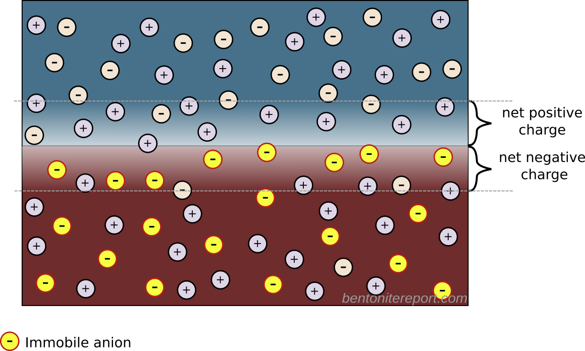
I find the statement regarding the advantage of reactive transport models highly problematic. Not only does it read more like an advertisement for the authors’ own tools than “fully developed text for self-study”, but the authors also seem ignorant of issues like the dangers of overparameterization (a theme that will recur).

“Classical Fickian Diffusion Theory”

As the title of the next section is “Classical Fickian Diffusion Theory,” a reader expects a discussion focused solely on diffusive process, especially when the immediate subtitle reads “Diffusion Basics.” I therefore find it peculiar that this section actually presents the traditional diffusion-sorption model, which describes a combination of diffusion and sorption processes. The model is summarized in eq. 10 in TS15

\begin{equation} \frac{\partial c}{\partial t} = \frac{D_e} {\phi + \rho_dK_D} \nabla ^ 2 c \end{equation}

where \(c\) is the “pore water” concentration of the considered species, \(D_e\) its “effective diffusivity”, \(K_D\) the sorption partition coefficient, \(\rho_d\) dry density, and \(\phi\) porosity.3 For later considerations we also note that TS15 define the denominator on the right hand side as the “rock capacity factor”, \(\alpha = \phi + \rho_dK_D\).

I find it particularly odd that two of the fundamental assumptions of this specific model are essentially left uncommented, namely that sorbed ions are immobilized and that the pores contain bulk water. Instead, the authors appear to question the assumption of Fickian diffusion in the context of clay systems, i.e. that diffusive fluxes are assumed proportional to corresponding aqueous concentration gradients.

This section aims, as far as I can see, to point out shortcomings in the description of diffusion in bentonite, and to motivate further model development. But it should be clear from the outset that using the traditional diffusion-sorption model as the basis for such an endeavor is doomed to fail. The reason for this failure is not due to assuming Fickian diffusion, but due to the other two model assumptions; it has long been demonstrated that exchangeable ions are mobile, and the notion that compacted bentonite contains mainly bulk water is absurd.

After the traditional diffusion-sorption model has been presented, it is evaluated by investigating how it can be fitted to tracer through-diffusion data (this is restatement of original work of Tachi and Yotsjui (2014)). Not surprisingly, it turns out that fitted diffusion coefficients may be unrealistically large. This is of course a direct consequence of the incorrect assumption of immobility in the traditional diffusion-sorption model. TS15 also appear to dismiss the model, saying

This result […] is not physically correct and points out the inconsistency of the classic Fickian diffusion theory for modeling diffusion processes in clay media.

I am bothered, though, that they keep using the phrase “classic Fickian diffusion theory”, which inevitably focuses on the Fickian aspect rather than on the obviously incorrect assumptions of the chosen model. Also, rather than simply concluding that the model is incorrect, TS15 continues4

[T]he large changes of \(\mathrm{Cs}^+\) diffusion parameters as a function of chemical conditions (\(D_{e,\mathrm{Cs}^+}\) decreases when the ionic strength increases […]) highlight the need to couple the chemical reactivity of clay materials to their transport properties in order to build reliable and predictive diffusion models.

There is no rationale for such a conclusion. I don’t even completely understand what “couple the chemical reactivity of clay materials to their transport properties” mean. Isn’t that what the traditional diffusion-sorption model attempts? What unrealistic \(D_e\) values actually highlights is simply that one should not use a model that assumes immobilization of “sorbed” ions.

To make things worse, TS15 describe the seeming uphill diffusion test and comment

However, the experimental observations were completely different: \(^{22}\mathrm{Na}^+\) accumulated in the high NaCl concentration reservoir as it was depleted in the low NaCl concentration reservoir, evidencing non-Fickian diffusion processes.

This is plain wrong. As explained in detail in an earlier post, the diffusion process in the “uphill” test is certainly Fickian. What the test demonstrates is, again, that “sorbed” ions are not immobile.

TS15 also comment on the results of fitting the model to anion tracer through-diffusion data. Here, as is well known, the fitted “rock capacity factor” \(\alpha = \phi + \rho_dK_D\) becomes significantly lower than the porosity \(\phi\). From the perspective of the traditional diffusion-sorption model, this is completely infeasible, as it implies a negative \(K_D\). But rather than simply dismissing the model, TS15 state

The lower \(\alpha\) values for anions than for water indicate that anions do not have access to all of the porosity.

Also this is incorrect. The porosity5 is an input parameter rather than a fitting parameter in the traditional diffusion-sorption model. When claiming that a small value of \(\alpha\) indicates a decreased porosity, TS15 reinterpret the parameter, on the fly, in terms of a completely different model: the effective porosity model. This model has not been mentioned at all earlier in the article.6

As has been discussed earlier on the blog, the effective porosity model can be fitted to anion tracer through-diffusion data, but now we need to keep track of two different models in the evaluation (something that TS15 do not). Moreover, these two models (the traditional diffusion-sorption and the effective porosity models) are incompatible. But TS15 continue by saying

This result is a first direct evidence of the limitation of the classic Fickian diffusion theory when applied to clay porous media: it is not possible to model the diffusion of water and anions with the same single porosity model. The observation of a lower \(\alpha\) value for anions than for water led to the development of the important concept of anion accessible porosity […]

This is a terrible passage. To begin with, the “Fickian” aspect is also here implied as the problem. But the reason for why the traditional diffusion-sorption model cannot be fitted to anion tracer through-diffusion data is of course because this model assumes the entire pore space to be filled with bulk water. Further, it’s hardly comprehensible what the authors mean by “it is not possible to model the diffusion of water and anions with the same single porosity model”. I think they simply mean that for water you must choose \(\alpha = \phi\), while for anion through-diffusion you instead must “choose” \(\alpha < \phi\). But the result \(\alpha < \phi\) should only lead to the conclusion that the traditional diffusion-sorption model cannot in any reasonable sense be fitted. A favorable reading of this passage is to assume that the authors actually mean that the effective porosity model can only be fitted to anion and water tracer through-diffusion data by using different values of the (effective) porosity, and that any “rock capacity factor” should not appear in this discussion.

Finally, the last sentence gives me headache. Rather than being an “important concept”, I mean that the idea of an “anion accessible porosity” has caused tremendous damage to the development of the bentonite research field for several decades now. We have earlier discussed on the blog that the whole idea of “anion accessible porosity” is based on misunderstandings. We have also demonstrated that the effective porosity model is not valid, even though it can be fitted to anion tracer through-diffusion data. A simple way to see this is to consider closed-cell diffusion data rather than through-diffusion data. Closed-cell tests are simpler than through-diffusion tests, as they don’t involve interfaces between clay and external solutions. We can e.g. take a look at the vast amount of diffusion coefficients for chloride in montmorillonite, presented in Kozaki et al. (1998).

There are in total 55(!) values, corresponding to 55(!) separate tests. These have been systematically varied with respect to density and temperature, but all of them were performed on montmorillonite equilibrated with distilled water. From the perspective of the effective porosity model, the effective porosity in such a system should be minute, perhaps even strictly zero; effective porosities evaluated from chloride through-diffusion tests are well below 1% even at a background concentration as large as 10 mM. Thus, if the idea of “anion accessible porosity” was reasonable, we’d expect extremely low values of the chloride diffusion coefficient in the above plot.7 We’d perhaps also expect a threshold behavior, where chloride diffusivity basically vanishes above a certain density. But this is not at all the behavior: chloride is seen to diffuse just fine in all 55(!) tests, with temperature- and density dependencies that seems reasonable for a homogeneous system. Moreover, chloride behaves very similarly to e.g. sodium, as seen here

Here the sodium data is from Kozaki et al. (1998),8 and it has also been measured in montmorillonite equilibrated with distilled water.

The effective porosity model and the notion of “anion accessible porosity” can consequently be dismissed directly, by comparing with simpler tests than what is done in TS15. The reason that the effective porosity model can be fitted to anion through-diffusion data must be attributed to a misinterpretation of such tests, as they involve also interfaces to external solutions. At least to me it is completely clear that what many researchers interpret as an effective porosity is actually effects of interface equilibrium.

If TS15 were serious about evaluating bentonite diffusion processes in this section I think they should have done the following:

  • Discuss the assumptions of ion immobility of sorbed ions and bulk pore water when presenting the traditional diffusion-sorption model. Moreover, they should not call this “Classical Fickian Diffusion Theory”.
  • Also present and discuss the effective porosity model, as they obviously use it in their evaluations. They actually even seem to promote it! And it is as “Fickian” as the traditional diffusion-sorption model.
  • Evaluate the models using closed-cell data to avoid misinterpretations arising from complications at bentonite/external solution interfaces.
  • Conclude that the traditional diffusion-sorption model is not valid for bentonite, and that this is because of the assumptions of immobility of sorbed ions and bulk pore water.
  • Conclude that the effective porosity model is not valid for bentonite, and that the notion of “anion accessible porosity” is flawed.

Instead, we get a quite confused and incomplete description, mixed with entirely inaccurate statements. In the end, it is difficult to understand what the takeaway message of this section really is. A reader is left with an impression that there is some problem with the “Fickian” aspect of diffusion, but nothing is spelled out. We have also been hinted that “anion accessible porosity” is important, without really having been introduced to the concept/model.

The section ends with the following passage

The limitations of the classic Fickian diffusion theory must find their origin in the fundamental properties of the clay minerals. In the next section, these fundamental properties are linked qualitatively to some of the observations described above.

If “classic Fickian diffusion theory” here is interpreted as “the traditional diffusion-sorption model” (which is literally what has been presented), the first sentence is both incorrect and trivial at the same time. The traditional diffusion-sorption model does not have “limitations” — it is fundamentally incorrect as a model for bentonite. The reason for this is that exchangeable ions are not immobile and that bentonite does not contain significant amounts of bulk water. Both of these reasons can be linked to “fundamental properties” of some specific clay minerals.

But it is clear that TS15 also have vaguely promoted the concept of “anion accessible porosity” and the effective porosity model. Are these not included in “the classic Fickian diffusion theory”? If not, why then is a model that assumes sorption and immobilization?

How can it not be immediately obvious to everyone that the diffusion process is much simpler than the contemporary descriptions?

As we have brought up the data from Kozaki et al. (1998), I would like to end this blog post by further considering actual profiles of chloride and sodium diffusing in montmorillonite.

This figure shows the corresponding normalized concentration profiles after 23.7 hours in closed-cell tests performed at \(50\;^\circ\mathrm{C}\) in Na-montmorillonite at dry density \(1.8 \;\mathrm{g/cm^3}\) that has been equilibrated with distilled water. In the case of sodium, both the profile evaluated from Fick’s second law (orange line) and measured values (circles) are plotted. In the case of chloride, no measured values are available, but the value of the diffusion coefficient is the result of fitting Fick’s second law (green line) to such data.

From the perspective of the traditional diffusion-sorption model, the sodium profile is supposed to represent the combined result of ions diffusing in bulk water, at a rate many orders of magnitude larger than in pure water, while being strongly retarded due to sorption onto “the solid” (where the ions are immobile). This is clearly nonsense, and something that I think TS15 actually tries to communicate.

From the perspective of the effective porosity model, on the other hand, the chloride profile is supposed to be the result of the ion diffusing in an essentially infinitesimal fraction of the pore volume, which magically is perfectly interconnected in all samples on which such tests are conducted. This is of course just as nonsensical as the above interpretation of the sodium profile, but in this case TS15 appear to promote the model (the “important concept of anion accessible porosity”).

Note that these two simple ions, at the end of the day, diffuse very similarly (please stop reading for a moment and contemplate the above plot). If sodium and chloride actually migrate in completely different domains and are subject to completely different physico-chemical processes, this “coincident” would be more than a little weird. Especially given that the two ions show similar diffusive behavior across a wide range of densities. To me, this simple observation makes it evident that ion diffusion in bentonite at the basic level is much simpler than what is suggested by the contemporary mainstream view. I mean that it is completely obvious that all ions in bentonite diffuse in the same type of quite homogeneous domain. And since it cannot be argued that the pore volume is dominated by anything other than interlayers at 1.8 g/cm³, this homogeneous domain is the interlayer domain at any relevant density. The evidence has been available for at least 25 years (in fact much longer than that). How can this be difficult to grasp?

Update (250213): Part II of this review is found here.

Footnotes

[1] By “bentonite” I here mean any type of smectite-rich system with a significant cation exchange capacity.

[2] The irony is that the “alternative” in a broader perspective is more mainstream than the “mainstream” view. I basically propose to obey the laws of thermodynamics.

[3] I have simplified the notation here somewhat compared with how it is written in TS15. As many others, TS15 call this equation “Fick’s second law” (via their eq. 4), which is not correct. Fick’s laws refer strictly to pure diffusion processes. However, the equation has the same form as Fick’s second law, if \(D_e/(\phi + \rho_d K_D)\) is treated as a single constant (often referred to as the apparent diffusivity).

[4] This behavior is of course not unique for cesium; I don’t know why TS15 focus so hard on that ion here.

[5] “Porosity” is a volume ratio. I’m not a fan of that the word has also begun to mean “pore space” in the bentonite scientific literature.

[6] In fact, \(\alpha\) has earlier in the article been unambiguously related to sorption:

If the species \(i\) is also adsorbed on or incorporated into the solid phase, then it is possible to define a rock capacity factor \(\alpha_i\) that relates the concentration in the porous media to the concentration in solution

[7] That the diffusivity is much too large for an effective porosity interpretation to make sense can also be seen from invoking Archie’s law, which is quite popular in bentonite scientific papers.

\begin{equation} D_e = \epsilon_\mathrm{eff}^n D_0\end{equation}

Here \(D_0\) is the diffusivity in pure bulk water, which is about \(2\cdot 10^{-9} \;\mathrm{m^2/s}\) for chloride. Using the popular choice \(n \approx 2\) and choosing e.g. \(\epsilon_\mathrm{eff} = 0.001\) (most probably an overestimation when using distilled water), we get

\begin{equation} D_0 = (5.1\cdot 10^{-11} \;\mathrm{m^2/s})/0.001 = 5.1\cdot 10^{-8} \;\mathrm{m^2/s}\end{equation}

This is more than twenty times the actual value for \(D_0\). (\(D_e = 5.1\cdot 10^{-14} \;\mathrm{m^2/s}\) is evaluated from Kozaki’s data at \(1.4 \;\mathrm{g/cm^3}\) and \(25\;^\circ\mathrm{C}\))

[8] Note! This publication is different from the chloride study.

“Uphill” diffusion in bentonite — a comment on Tertre et al. (2024)

The vast majority of published tests on ion diffusion in bentonite deal with chemically uniform systems, and in a previous blog post I addressed the lack of studies where actual chemical gradients are maintained. But recently such a study was published: “Influence of salinity gradients on the diffusion of water and ionic species in dual porosity clay samples” (Tertre et al., 2024). Although I’m pleased to see these types of experiments being reported, I must admit that the paper as a whole leaves me quite disappointed.

The paper follows a structure recognizable from several others that we have considered previously on the blog: It starts off with an introduction section containing several incorrect or unfounded statements1 regarding bentonite.2 It then presents some experimental results that makes it evident that no real progress has been made for a long time regarding e.g. experimental design.3 The major part of the paper is devoted to a “results and discussion” section with several incorrect statements and inferences, speculation, and irrelevant modeling.

Here I would like to focus on how the study “Seeming steady-state uphill diffusion of \(^{22}\mathrm{Na}^+\) in compacted montmorillonite” (Glaus et al., 2013) is referenced:

[I]nfluence of a background electrolyte concentration gradient on the diffusion of anionic and cationic species at trace concentrations has […] been rarely investigated. Notable exceptions are the DR-A in situ diffusion experiment conducted at the Mont-Terri laboratory (Soler et al., 2019), and an “uphill” diffusion experiment of a \(^{22}\mathrm{Na}^+\) tracer in a compacted sodium montmorillonite (Glaus et al., 2013). These two studies demonstrated the marked influence of background electrolyte concentration gradient on tracer diffusion, and thus the necessity to understand the couplings between diffusion of several charged species present at contrasting concentrations and experiencing different concentration gradients. The experiment from Glaus et al. (2013) also demonstrated the importance of considering diffusion processes occurring in the porosity next to the charged surface of clay minerals (i.e., the porosity associated to the EDL of particles).

This quotation contains two statements relating to Glaus et al. (2013), both of which I think are problematic4

  • It basically claims that the “uphill” phenomenon is due to diffusive couplings between several types of ions. Of course, ion diffusion always involves couplings between different types of ions, due to the requirement of electroneutrality. But it is clear that Tertre et al. (2024) mean that the “uphill” effect is caused by additional couplings that are not present in chemically homogeneous systems.
  • It says that Glaus et al. (2013) demonstrates the importance to consider diffuse layers. I agree with this, but it is written in a way that implies that there also are other relevant “porosities”, and that there are other types of tests where ion diffusion in bentonite is not significantly influenced by the presence of diffuse layers.

As one of the authors of the “uphill” study, I would here like to argue for why I think the above statements are problematic and give some background context.

The “uphill” diffusion experiment

The “uphill” study actually originated from a prediction presented by me in a conference poster session. This poster discussed the role of the quantity \(D_e\), using the exact same theory that we had previously used to explain the diffusive behavior of tracer ions in compacted bentonite as an effect of Donnan equilibrium in a homogeneous system. In particular, it pointed out that \(D_e\) — although universally referred to as the (effective) “diffusion coefficient” — is not a diffusion coefficient in the context of compacted bentonite. I have continued this discussion in later papers, and in several posts on this blog.

In the poster, we suggested the “uphill” experiment as a demonstration of the shortcoming of \(D_e\). If the two reservoirs in a through-diffusion test are maintained at different background concentrations, the theory predicts a non-zero tracer flux for a vanishing external tracer concentration difference, i.e. an “infinite” value of \(D_e\). The suggestion caught the interest of an experimental group, and after a successful collaboration we could present the results of an actual “uphill” experiment. Without making too much of an exaggeration, I would say that the results of this experiment were basically exactly as predicted.

Given this background, it should be clear that the tests in Glaus et al. (2013) follow exactly the same rules as tests in chemically homogeneous systems, rather than demonstrating “the necessity to understand the couplings between diffusion of several charged species present at contrasting concentrations”. Although it is quite clearly stated already in the abstract in Glaus et al. (2013), there is apparently still a need to communicate this explanation. Let me therefore try that here.

The “uphill” diffusion phenomenon explained

Consider an ordinary aqueous solution containing radioactive \(^{22}\mathrm{Na}\) and stable \(^{23}\mathrm{Na}\). The fraction of \(^{22}\mathrm{Na}\) ions can be written \(c_\mathrm{ext}/C_\mathrm{bkg}\), where \(c_\mathrm{ext}\) is the \(^{22}\mathrm{Na}\) concentration, and \(C_\mathrm{bkg}\) is the total sodium concentration (the “tracer” and “background” concentrations, respectively).

Since \(^{23}\mathrm{Na}\) and \(^{22}\mathrm{Na}\) are basically chemically indistinguishable, the same \(^{22}\mathrm{Na}\)-fraction will be maintained in any system with which this solution is in equilibrium. In particular, if the solution is in equilibrium with a montmorillonite interlayer solution, we can write

\begin{equation*} \frac{c_\mathrm{int}}{C_\mathrm{int}} = \frac{c_\mathrm{ext}}{C_\mathrm{bkg}} \tag{1} \end{equation*}

where \(c_\mathrm{int}\) and \(C_\mathrm{int}\) are the \(^{22}\mathrm{Na}\) and total interlayer concentrations, respectively. The total interlayer cation concentration (\(C_\mathrm{int}\)) can be handled in different ways, but it is important to note that this is a substantial number under all conditions, relating to the cation exchange capacity.5 Rearranging eq. 1 gives

\begin{equation*} c_\mathrm{int} = \frac{C_\mathrm{int}}{C_\mathrm{bkg}}\cdot c_\mathrm{ext} \end{equation*}

Since the interlayer cation concentration is always larger than the corresponding background concentration, the above equation tells us that the corresponding interlayer tracer concentration becomes enhanced, by the factor \(C_\mathrm{int}/C_\mathrm{bkg}\).

Conventional through-diffusion

This enhancement mechanism causes the diffusional behavior of \(^{22}\mathrm{Na}\) in conventional through-diffusion experiments in bentonite. In such experiments, the tracer concentration in the target reservoir is usually kept near zero, and the actual steady-state concentration gradient in the interlayers is

\begin{equation*} \frac{\partial c_\mathrm{int}}{\partial x} = \frac{0- C_\mathrm{int}/C_\mathrm{bkg}\cdot c_\mathrm{ext}^{(1)}} {L} = -\frac{C_\mathrm{int}}{C_\mathrm{bkg}}\cdot \frac{ c_\mathrm{ext}^{(1)} }{ L } \end{equation*}

where we have indexed the tracer concentration in the source reservoir with “\((1)\)”, labeled the sample length \(L\), and assumed that ions diffuse in the \(x\)-direction. The corresponding flux is thus (Fick’s law)

\begin{equation*} j_\mathrm{steady-state} = – \phi D_c\frac{\partial c_\mathrm{int}}{\partial x} = \phi D_c\cdot \frac{C_\mathrm{int}}{C_\mathrm{bkg}}\cdot \frac{c_\mathrm{ext}^{(1)} } {L} \tag{2} \end{equation*}

where \(D_c\) denotes the (macroscopic) diffusivity in the interlayers, and \(\phi\) is porosity. Keeping \(c_\mathrm{ext}^{(1)}\) constant, eq. 2 shows that the \(^{22}\mathrm{Na}\) steady-state flux increases indefinitely as the background concentration is made small, in full agreement with experimental observation.6

The picture below illustrates the concentration conditions in an conventional through-diffusion test.

Here we have chosen \(C_\mathrm{int}=\) 4.0 M, the background concentration in the two reservoirs (blue) is put equal to 0.1 M, and the tracer concentration (orange) is put to 0.1 mM in reservoir 1 (and zero i reservoir 2). The corresponding internal tracer gradient is plotted in the right side diagram, and the resulting diffusive flux is indicated by the arrow.

“Uphill” diffusion

To explain the “uphill” effect the only modifications needed in the above derivation is to allow for different background concentrations in the external reservoirs, and to recognize that the tracer concentration in the clay on the “target” side (indexed “\((2)\)”) no longer is zero. Considering the tracer concentration enhancement at both interfaces, the steady-state interlayer concentration gradient then reads

\begin{equation*} \frac{\partial c_\mathrm{int}}{\partial x} = \frac{ C_\mathrm{int}/C_\mathrm{bkg}^{(2)}\cdot c_\mathrm{ext}^{(2)} -C_\mathrm{int}/C_\mathrm{bkg}^{(1)}\cdot c_\mathrm{ext}^{(1)}} {L} \end{equation*}

To be more concrete, let’s assume that \(C_\mathrm{bkg}^{(2)} = 5\cdot C_\mathrm{bkg}^{(1)}\), which is the same ratio as in Glaus et al. (2013). We then have

\begin{equation*} \frac{\partial c_\mathrm{int}}{\partial x} = \frac{C_\mathrm{int}}{C_\mathrm{bkg}^{(1)}} \cdot \frac{ c_\mathrm{ext}^{(2)}/5 – c_\mathrm{ext}^{(1)}} {L} \end{equation*}

giving the corresponding steady-state flux

\begin{equation*} j_\mathrm{steady-state} = \phi D_c\cdot \frac{C_\mathrm{int}}{C_\mathrm{bkg}^{(1)}} \cdot \frac{ c_\mathrm{ext}^{(1)} – c_\mathrm{ext}^{(2)}/5} {L} \end{equation*}

Note that we recover the conventional through-diffusion result (eq. 2) from this expression, if we put \(c_\mathrm{ext}^{(2)}= 0\). But if we e.g. set the tracer concentration equal in both reservoirs, we still have a flux from side \((1)\) to side \((2)\), of size \(j = 4/5 \cdot \phi D_c\cdot C_\mathrm{int}/C_\mathrm{bkg}^{(1)}\cdot c_\mathrm{ext}^{(1)}\). And even if we make \(c_\mathrm{ext}^{(2)}\) larger than \(c_\mathrm{ext}^{(1)}\) — as long as \(c_\mathrm{ext}^{(1)}< c_\mathrm{ext}^{(2)} < 5\cdot c_\mathrm{ext}^{(1)}\) — we still have a diffusive flux from side \((1)\) to side \((2)\), i.e seeming “uphill” diffusion.

Below is illustrated the concentration conditions in an “uphill” configuration.

In contrast to the above illustration for conventional through-diffusion, the background concentration in reservoir 2 is here raised to 0.5 M and the tracer concentration in reservoir 2 is put equal to 0.2 mM. We see that, although tracers are transported to the reservoir with higher concentration, the process is still ordinary Fickian diffusion, as the internal tracer gradient has the same direction as in the conventional case.

We can now conclude what was stated above: The “uphill” diffusion effect is caused by exactly the same mechanism that cause the behavior of cation diffusion in conventional bentonite through-diffusion tests. This mechanism is ion equilibrium between clay and external solutions at the two interfaces. In this particular case, with sodium tracers diffusing in a sodium background, we don’t need to invoke the full ion equilibrium framework in order to quantify the fluxes, but can rely on the very robust result that any two systems in equilibrium have the same tracer fraction (eq. 1).

Reexamining the Tertre et al. (2024) statements

With the explanation for the “uphill” effect established, let’s re-examine the problematic statements in Tertre et al. (2024) identified above

  • Glaus et al. (2013) cannot be used to support a claim of “marked influence” of additional diffusional couplings. The opposite is true: Glaus et al. (2013) found no significant influence from mechanisms beyond those in chemically homogeneous conditions.
  • The “uphill” effect was predicted from taking the idea seriously that diffusion in compacted bentonite is fully governed by interlayer properties. Singling out Glaus et al. (2013) as the study that demonstrates the importance of diffuse layers7 therefore gives the wrong impression. Rather, what Glaus et al. (2013) demonstrates, in conjunction with corresponding conventional through-diffusion results, is that compacted bentonite contains insignificant amounts of bulk water (what Tertre et al. (2024) call “interparticle water”).

A way forward (if anybody cares)

After the uphill study was published I was for a while under the illusion that things would begin to change within the compacted bentonite research field. Not only did the study, to my mind, deal a fatal blow to any bentonite model that relies on the presence of a bulk water phase in the clay. It also opened up a whole new area of interesting studies to conduct. Now, some 11 years later, I can disappointingly conclude that not a single additional study has been presented that explore the ideas here discussed.8 And, regarding bentonite models, bulk water is apparently alive and kicking, as has been discussed ad nauseum on this blog.

Experimentally, there are a number of interesting questions looking for answers. In particular, we actually do expect additional mechanisms to play a role in chemically inhomogeneous systems, e.g. osmosis, and other effects due to presence of salt concentration gradients and electrostatic potential differences. It may be argued for why such effects are not significant in Glaus et al. (2013), but it is of course both of fundamental and practical interest to understand under which conditions they are. The original “uphill” study is e.g. performed at quite extreme density (\(1900\;\mathrm{m^3/kg}\)). How would the result differ at \(1600\;\mathrm{m^3/kg}\) or \(1300\;\mathrm{m^3/kg}\)? Also, how would the results change with other choices of the reservoir concentrations, and how would the results differ if one of the cations is not at trace level (e.g. a system with comparable amounts of sodium and potassium)?

Even under the conditions of the original study, there are several predictions left to verify. If e.g. \(c^{(1)}_\mathrm{ext} = c^{(2)}_\mathrm{ext}/5\), the theory predicts zero flux (implying \(D_e = 0\)). The theory also implies that when performing “conventional” through-diffusion, the actual level of the background concentration in the target reservoir is irrelevant, as long as the tracer concentration is kept at zero.

In fact, one can imagine making a whole cycle of through-diffusion tests to explore the ideas here discussed, as illustrated in this animation

The resulting steady-state flux for various external conditions is indicated by the arrow. Here, the full ion equilibrium framework was used to calculate the internal concentrations (giving an internal gradient also in \(C_\mathrm{int}\)). Background concentrations and total interlayer concentration is chosen to be comparable with Glaus et al. (2013), while the choice for tracer concentration is arbitrary.9

With the risk of sounding hubristic, the number of experiments suggested in the above animation could have given enough material for several Ph.D. theses. But here we are, in the year 2024, without even a replication of the “uphill” effect. Instead, a basically entire research field has been stuck for decades with the ludicrous idea that models of compacted bentonite should be based on a bulk water description. I find this both hilarious and horrific.

Update (260803): A further treatment of the “uphill” test with focus on the electrostatic potential is found here.

Footnotes

[1] For example (follow links to discussions on these issues):

  • It states the traditional diffusion-sorption model as being relevant in these systems. It is not.
  • It somehow manages to combine the traditional diffusion-sorption model with the effective porosity model for anion tracer diffusion, although these two models are incompatible.
  • Related to using the traditional diffusion-sorption model, it assumes \(D_e\) to be a real diffusion coefficient, which it is not. I find this particularly remarkable in a paper that deals with the presence of “saline gradients”. A motivation behind e.g. the “uphill” test is to point out the shortcomings of \(D_e\), as discussed in the rest of this blog post.
  • It claims that “anionic and cationic tracers do not experience the same overall accessible porosity”, which is unjustified.
  • It claims that “diffusion rates” of anions are decreased and “diffusion rates” of cations are increased, compared to “neutral species”, due to different interactions with diffuse layers. But this is not true generally.
  • It implicitly simply assumes a “stack”-view of these clay systems. But stacks don’t make much sense.

[2] I use the word “bentonite” here quite loosely. Tertre et al. (2024) use wordings such as “clayey samples”, “argillaceous rocks” and “clayey formation”, but it is clear that the presented material is supposed to apply to actual bentonite.

[3] I’m specifically thinking about that cation tracer through-diffusion tests at low background concentration is not a good idea, and that it is completely clear from the results presented in Tertre et al. (2024) that some of these are mainly controlled by diffusion in the confining filters. Estimating a “rock capacity factor” larger than 750 for sodium tracers in a sodium-clay (at 20 mM background concentration) should have set off all alarm bells.

[4] Regarding Soler et al. (2019), I think that whole study is problematic, which I might argue for in a separate blog post.

[5] Glaus et al. (2013) invoke the “exchange site” activity \([\mathrm{NaX}]\) to discuss this quantity. I personally prefer relating it to the quantity \(c_\mathrm{IL}\) that is defined within the homogeneous mixture model.

[6] This agreement has been shown to be quantitative, see e.g. Glaus et al. (2007), Birgersson and Karnland (2009) and Birgersson (2017). Note that this result is quite independent of how many “porosities” you choose to include in a model; it’s merely a consequence of treating the dominating pores (interlayers) adequately. Further, note that measuring the diverging fluxes in the limit of low background concentration becomes increasingly difficult, as the confining filters becomes rate limiting.

[7] In the present context, I presume the terms “diffuse layer” and “interlayer” to be more or less equivalent. Other authors instead make an unjustified distinction, that I have addressed here.

[8] There are a few examples of published studies where effects of the kind discussed here are present, but where the authors don’t seem to be aware of it.

[9] Tracer concentrations in Glaus et al. (2013) is much smaller, but this value does not affect any behavior, as long as it is small in comparison with total concentration.

Are interlayer cations not attracted to the surfaces?!

Electrostatics can be quite subtle. The following comment on the interlayer ion distribution, in Kjellander et al. (1988), was an eye-opener for me

The ion concentration profile is determined by the net force acting on each ion. The electrostatic potential from the uniform surface charges is constant between the two walls, which means that the forces due to these charges cancel each other completely. Thus, the large counter-ion concentration in the electric double layer near the walls is solely a consequence of the repulsive interactions between the ions.

Interlayer cations are not attracted to the surfaces, but are pushed towards them due to repulsion between the ions themselves! My intuition has been that interlayer counter-ions distribute due to attraction with the surfaces, but the perspective given in the above quotation certainly makes a lot of sense. Here I use the word “perspective” because I don’t fully agree with the statement that the ion distribution is solely a consequence of repulsion. To discuss the issue further, let’s flesh out the reasoning in Kjellander et al. (1988) and draw some pictures.

Here we discuss an idealized model of an interlayer as a dielectric continuum sandwiched between two parallel infinite planes of uniform surface charge density.1 The system is thus symmetric around the axis normal to the surfaces (the model is one-dimensional).

From electrostatics we know that the electric field originating from a plane of uniform surface charge has the same size at any distance from the plane (we discussed this fact in the blog post on electrostatics and swelling pressure). We may draw such electric fields like this

From this result follows that the electric field vanishes between two equally negatively charged surfaces. The electrostatic field configuration for an “empty” interlayer can thus be illustrated like this

This means that the two interlayer surfaces don’t “care” about the counter-ions, in the sense that this part of the electrostatic energy (ion – surfaces) is independent of the counter-ion distribution.

To consider the fate of the counter-ions we continue to explore the axial symmetry. The counter-ion distribution varies only in the direction normal to the surfaces, and we can treat it as a sequence of thin parallel planes of uniform charge. Since the size of the electric field from such planes is independent of distance, the force on a positive test charge (= the electric field) at any position in the interlayer depends only on the difference in total amount of charge on each side of this position, as illustrated here

This, in turn, implies both that the electric field is zero at the mid position, and that the electric field elsewhere is directed towards the closest surface (since symmetry requires equal amount of charge in the two halves of the interlayer2). The counter-ions indeed repel each other towards the surfaces! The charge density must therefore increase towards the surfaces, and we understand that the equilibrium electric field qualitatively must look like this3

However, as far as I see, the “indifference” of the surfaces to the counter-ions is a matter of perspective. Consider e.g. making the interlayer distance very large. In this limit, the system is more naturally conceptualized as two single surfaces. It is then awkward to describe the ion distribution at one surface as caused by repulsion from other ions arbitrarily far away, rather than as caused by attraction to the surface. But for the case most relevant for compacted bentonite — i.e. interlayers, or what is often described as “overlapping” electric double layers — the natural perspective is that counter-ions distribute as a consequence of repulsion among themselves.

This perspective also implies that anions (co-ions) distribute within the interlayer as a consequence of attraction to counter-ions rather than repulsion from the surfaces! (The above figure applies, with all arrows reversed.) This insight should not be confused with the fact that repulsion between anions and surfaces is not really the mechanism behind “anion exclusion”. Rather, the implication here is that anion-surface repulsion can be viewed as not even existing within an interlayer.

A couple of corrections

With this (to me) new perspective in mind, I’d like to correct a few formulations in the blog post on electrostatics and swelling. In that post, I write

[R]ather than contributing to repulsion, electrostatic interactions actually reduce the pressure. This is clearly seen from e.g. the Poisson-Boltzmann solution for two charged surfaces, where the resulting osmotic pressure corresponds to an ideal solution with a concentration corresponding to the value at the midpoint (cf. the quotation from Kjellander et al. (1988) above). But the midpoint concentration — and hence the osmotic pressure — is lowered as compared with the average, because of electrostatic attraction between layers and counter-ions.

But the final sentence should rather be formulated as

But the midpoint concentration — and hence the osmotic pressure — is lowered as compared with the average, because of electrostatic repulsion between the counter-ions.

In the original post, I also write

This plot demonstrates the attractive aspect of electrostatic interactions in these systems. While the NaCl pressure is only slightly reduced, Na-montmorillonite shows strong non-ideal behavior. In the “low” concentration regime (< 2 mol/kgw) we understand the pressure reduction as an effect of counter-ions electrostatically attracted to the clay surfaces.

The last part is better formulated as

In the “low” concentration regime (< 2 mol/kgw) we understand the pressure reduction as an effect of electrostatic repulsion among the counter-ions.

I think the implication here is quite wild: In a sense, electrostatic repulsion reduces swelling pressure!

Footnotes

[1] The treatment in Kjellander et al. (1988) is more advanced, including effects of image charges and ion-ion correlations, but it does not matter for the present discussion.

[2] Actually, the whole distribution is required to be symmetric around the interlayer midpoint.

[3] The quantitative picture is of course achieved from solving the Poisson-Boltzmann equation. The picture may be altered when considering more involved mechanisms, such as image charge interactions or ion-ion correlations; Kjellander et al. (1988) show that the effect of image charges may reduce the ion distribution at very short distances, while the effect of ion-ion correlations is to further increase the accumulation towards the surfaces. Note that neither of these effects involve direct interaction with the surface charge.

Multi-porosity models cannot be taken seriously (Semi-permeability, part II)

“Multi-porosity” models1 — i.e models that account for both a bulk water phase and one, or several, other domains within the clay — have become increasingly popular in bentonite research during the last couple of decades. These are obviously macroscopic, as is clear e.g. from the benchmark simulations described in Alt-Epping et al. (2015), which are specified to be discretized into 2 mm thick cells; each cell is consequently assumed to contain billions and billions individual montmorillonite particles. The macroscopic character is also relatively clear in their description of two numerical tools that have implemented multi-porosity

PHREEQC and CrunchFlowMC have implemented a Donnan approach to describe the electrical potential and species distribution in the EDL. This approach implies a uniform electrical potential \(\varphi^\mathrm{EDL}\) in the EDL and an instantaneous equilibrium distribution of species between the EDL and the free water (i.e., between the micro- and macroporosity, respectively). The assumption of instantaneous equilibrium implies that diffusion between micro- and macroporosity is not considered explicitly and that at all times the chemical potentials, \(\mu_i\), of the species are the same in the two porosities

On an abstract level, we may thus illustrate a multi-porosity approach something like this (here involving two domains)

The model is represented by one continuum for the “free water”/”macroporosity” and one for the “diffuse layer”/”microporosity”,2 which are postulated to be in equilibrium within each macroscopic cell.

But such an equilibrium (Donnan equilibrium) requires a semi-permeable component. I am not aware of any suggestion for such a component in any publication on multi-porosity models. Likewise, the co-existence of diffuse layer and free water domains requires a mechanism that prevents swelling and maintains the pressure difference — also the water chemical potential should of course be the equal in the two “porosities”.3

Note that the questions of what constitutes the semi-permeable component and what prevents swelling have a clear answer in the homogeneous mixture model. This answer also corresponds to an easily identified real-world object: the metal filter (or similar component) separating the sample from the external solution. Multi-porosity models, on the other hand, attribute no particular significance to interfaces between sample and external solutions. Therefore, a candidate for the semi-permeable component has to be — but isn’t — sought elsewhere. Donnan equilibrium calculations are virtually meaningless without identifying this component.

The partitioning between diffuse layer and free water in multi-porosity models is, moreover, assumed to be controlled by water chemistry, usually by means of the Debye length. E.g. Alt-Epping et al. (2015) write

To determine the volume of the microporosity, the surface area of montmorillonite, and the Debye length, \(D_L\), which is the distance from the charged mineral surface to the point where electrical potential decays by a factor of e, needs to be known. The volume of the microporosity can then be calculated as \begin{equation*}
\phi^\mathrm{EDL} = A_\mathrm{clay} D_L, \end{equation*} where \(A_\mathrm{clay}\) is the charged surface area of the clay mineral.

I cannot overstate how strange the multi-porosity description is. Leaving the abstract representation, here is an attempt to illustrate the implied clay structure, at the “macropore” scale

The view emerging from the above description is actually even more peculiar, as the “micro” and “macro” volume fractions are supposed to vary with the Debye length. A more general illustration of how the pore structure is supposed to function is shown in this animation (“I” denotes ionic strength)

What on earth could constitute such magic semi-permeable membranes?! (Note that they are also supposed to withstand the inevitable pressure difference.)

Here, the informed reader may object and point out that no researcher promoting multi-porosity has this magic pore structure in mind. Indeed, basically all multi-porosity publications instead vaguely claim that the domain separation occurs on the nanometer scale and present microscopic illustrations, like this (this is a simplified version of what is found in Alt-Epping et al. (2015))

In the remainder of this post I will discuss how the idea of a domain separation on the microscopic scale is even more preposterous than the magic membranes suggested above. We focus on three aspects:

  • The implied structure of the free water domain
  • The arbitrary domain division
  • Donnan equilibrium on the microscopic scale is not really a valid concept

Implied structure of the free water domain

I’m astonished by how little figures of the microscopic scale are explained in many publications. For instance, the illustration above clearly suggests that “free water” is an interface region with exactly the same surface area as the “double layer”. How can that make sense? Also, if the above structure is to be taken seriously it is crucial to specify the extensions of the various water layers. It is clear that the figure shows a microscopic view, as it depicts an actual diffuse layer.4 A diffuse layer width varies, say, in the range 1 – 100 nm,5 but authors seldom reveal if we are looking at a pore 1 nm wide or several hundred nm wide. Often we are not even shown a pore — the water film just ends in a void, as in the above figure.6

The vague nature of these descriptions indicates that they are merely “decorations”, providing a microscopic flavor to what in effect still is a macroscopic model formulation. In practice, most multi-porosity formulations provide some ad hoc mean to calculate the volume of the diffuse layer domain, while the free water porosity is either obtained by subtracting the diffuse layer porosity from total porosity, or by just specifying it. Alt-Epping et al. (2015), for example, simply specifies the “macroporosity”

The total porosity amounts to 47.6 % which is divided into 40.5 % microporosity (EDL) and 7.1 % macroporosity (free water). From the microporosity and the surface area of montmorillonite (Table 7), the Debye length of the EDL calculated from Eq. 11 is 4.97e-10 m.

Clearly, nothing in this description requires or suggests that the “micro” and “macroporosities” are adjacent waterfilms on the nm-scale. On the contrary, such an interpretation becomes quite grotesque, with the “macroporosity” corresponding to half a monolayer of water molecules! An illustration of an actual pore of this kind would look something like this

This interpretation becomes even more bizarre, considering that Alt-Epping et al. (2015) assume advection to occur only in this half-a-monolayer of water, and that the diffusivity is here a factor 1000 larger than in the “microporosity”.

As another example, Appelo and Wersin (2007) model a cylindrical sample of “Opalinus clay” of height 0.5 m and radius 0.1 m, with porosity 0.16, by discretizing the sample volume in 20 sections of width 0.025 m. The void volume of each section is consequently \(V_\mathrm{void} = 0.16\cdot\pi\cdot 0.1^2\cdot 0.025\;\mathrm{m^3} = 1.257\cdot10^{-4}\;\mathrm{m^3}\). Half of this volume (“0.062831853” liter) is specified directly in the input file as the volume of the free water;7 again, nothing suggests that this water should be distributed in thin films on the nm-scale. Yet, Appelo and Wersin (2007) provide a figure, with no length scale, similar in spirit to that above, that look very similar to this

They furthermore write about this figure (“Figure 2”)

It should be noted that the model can zoom in on the nm-scale suggested by Figure 2, but also uses it as the representative form for the cm-scale or larger.

I’m not sure I can make sense of this statement, but it seems that they imply that the illustration can serve both as an actual microscopic representation of two spatially separated domains and as a representation of two abstract continua on the macroscopic scale. But this is not true!

Interpreted macroscopically, the vertical dimension is fictitious, and the two continua are in equilibrium in each paired cell. On a microscopic scale, on the other hand, equilibrium between paired cells cannot be assumed a priori, and it becomes crucial to specify both the vertical and horizontal length scales. As Appelo and Wersin (2007) formulate their model assuming equilibrium between paired cells, it is clear that the above figure must be interpreted macroscopically (the only reference to a vertical length scale is that the “free solution” is located “at infinite distance” from the surface).

We can again work out the implications of anyway interpreting the model microscopically. Each clay cell is specified to contain a surface area of \(A_\mathrm{surf}=10^5\;\mathrm{m^2}\).8 Assuming a planar geometry, the average pore width is given by (\(\phi\) denotes porosity and \(V_\mathrm{cell}\) total cell volume)

\begin{equation} d = 2\cdot \phi \cdot \frac{V_\mathrm{cell}}{A_\mathrm{surf}} = 2\cdot \frac{V_\mathrm{void}}{A_\mathrm{surf}} = 2\cdot \frac{1.26\cdot 10^{-4}\;\mathrm{m^3}}{10^{5}\;\mathrm{m^2}} = 2.51\;\mathrm{nm} \end{equation}

The double layer thickness is furthermore specified to be 0.628 nm.9 A microscopic interpretation of this particular model thus implies that the sample contains a single type of pore (2.51 nm wide) in which the free water is distributed in a thin film of width 1.25 nm — i.e. approximately four molecular layers of water!

Rather than affirming that multi-porosity model formulations are macroscopic at heart, parts of the bentonite research community have instead doubled down on the confusing idea of having free water distributed on the nm-scale. Tournassat and Steefel (2019) suggest dealing with the case of two parallel charged surfaces in terms of a “Dual Continuum” approach, providing a figure similar to this (surface charge is -0.11 C/m2 and external solution is 0.1 M of a 1:1 electrolyte)

Note that here the perpendicular length scale is specified, and that it is clear from the start that the electrostatic potential is non-zero everywhere. Yet, Tournassat and Steefel (2019) mean that it is a good idea to treat this system as if it contained a 0.7 nm wide bulk water slice at the center of the pore. They furthermore express an almost “postmodern” attitude towards modeling, writing

It should be also noted here that this model refinement does not imply necessarily that an electroneutral bulk water is present at the center of the pore in reality. This can be appreciated in Figure 6, which shows that the Poisson–Boltzmann predicts an overlap of the diffuse layers bordering the two neighboring surfaces, while the dual continuum model divides the same system into a bulk and a diffuse layer water volume in order to obtain an average concentration in the pore that is consistent with the Poisson–Boltzmann model prediction. Consequently, the pore space subdivision into free and DL water must be seen as a convenient representation that makes it possible to calculate accurately the average concentrations of ions, but it must not be taken as evidence of the effective presence of bulk water in a nanoporous medium.

I can only interpret this way of writing (“…does not imply necessarily that…”, “…must not be taken as evidence of…”) that they mean that in some cases the bulk phase should be interpreted literally, while in other cases the bulk phase should be interpreted just as some auxiliary component. It is my strong opinion that such an attitude towards modeling only contributes negatively to process understanding (we may e.g. note that later in the article, Tournassat and Steefel (2019) assume this perhaps non-existent bulk water to be solely responsible for advective flow…).

I say it again: no matter how much researchers discuss them in microscopic terms, these models are just macroscopic formulations. Using the terminology of Tournassat and Steefel (2019), they are, at the end of the day, represented as dual continua assumed to be in local equilibrium (in accordance with the first figure of this post). And while researchers put much effort in trying to give these models a microscopic appearance, I am not aware of anyone suggesting a reasonable candidate for what actually could constitute the semi-permeable component necessary for maintaining such an equilibrium.

Arbitrary division between diffuse layer and free water

Another peculiarity in the multi-porosity descriptions showing that they cannot be interpreted microscopically is the arbitrary positioning of the separation between diffuse layer and free water. We saw earlier that Alt-Epping et al. (2015) set this separation at one Debye length from the surface, where the electrostatic potential is claimed to have decayed by a factor of e. What motivates this choice?

Most publications on multi-porosity models define free water as a region where the solution is charge neutral, i.e. where the electrostatic potential is vanishingly small.10 At the point chosen by Alt-Epping et al. (2015), the potential is about 37% of its value at the surface. This cannot be considered vanishingly small under any circumstance, and the region considered as free water is consequently not charge neutral.

The diffuse layer thickness chosen by Appelo and Wersin (2007) instead corresponds to 1.27 Debye lengths. At this position the potential is about 28% of its value at the surface, which neither can be considered vanishingly small. At the mid point of the pore (1.25 nm), the potential is about 8%11 of the value at the surface (corresponding to about 2.5 Debye lengths). I find it hard to accept even this value as vanishingly small.

Note that if the boundary distance used by Appelo and Wersin (2007) (1.27 Debye lengths) was used in the benchmark of Alt-Epping et al. (2015), the diffuse layer volume becomes larger than the total pore volume! In fact, this occurs in all models of this kind for low enough ionic strength, as the Debye length diverges in this limit. Therefore, many multi-porosity model formulations include clunky “if-then-else” clauses,12 where the system is treated conceptually different depending on whether or not the (arbitrarily chosen) diffuse layer domain fills the entire pore volume.13

In the example from Tournassat and Steefel (2019) the extension of the diffuse layer is 1.6 nm, corresponding to about 1.69 Debye lengths. The potential is here about 19% of the surface value (the value in the midpoint is 12% of the surface value). Tournassat and Appelo (2011) uses yet another separation distance — two Debye lengths — based on misusing the concept of exclusion volume in the Gouy-Chapman model.

With these examples, I am not trying to say that a better criterion is needed for the partitioning between diffuse layer and bulk. Rather, these examples show that such a partitioning is quite arbitrary on a microscopic scale. Of course, choosing points where the electrostatic potential is significant makes no sense, but even for points that could be considered having zero potential, what would be the criterion? Is two Debye lengths enough? Or perhaps four? Why?

These examples also demonstrate that researchers ultimately do not have a microscopic view in mind. Rather, the “microscopic” specifications are subject to the macroscopic constraints. Alt-Epping et al. (2015), for example, specifies a priori that the system contains about 15% free water, from which it follows that the diffuse layer thickness must be set to about one Debye length (given the adopted surface area). Likewise, Appelo and Wersin (2007) assume from the start that Opalinus clay contains 50% free water, and set up their model accordingly.14 Tournassat and Steefel (2019) acknowledge their approach to only be a “convenient representation”, and don’t even relate the diffuse layer extension to a specific value of the electrostatic potential.15 Why the free water domain anyway is considered to be positioned in the center of the nanopore is a mystery to me (well, I guess because sometimes this interpretation is supposed to be taken literally…).

Note that none of the free water domains in the considered models are actually charged, even though the electrostatic potential in the microscopic interpretations is implied to be non-zero. This just confirms that such interpretations are not valid, and that the actual model handling is the equilibration of two (or more) macroscopic, abstract, continua. The diffuse layer domain is defined by following some arbitrary procedure that involves microscopic concepts. But just because the diffuse layer domain is quantified by multiplying a surface area by some multiple of the Debye length does not make it a microscopic entity.4

Donnan effect on the microscopic scale?!

Although we have already seen that we cannot interpret multi-porosity models microscopically, we have not yet considered the weirdest description adopted by basically all proponents of these models: they claim to perform Donnan equilibrium calculations between diffuse layer and free water regions on the microscopic scale!

The underlying mechanism for a Donnan effect is the establishment of charge separation, which obviously occur on the scale of the ions, i.e. on the microscopic scale. Indeed, a diffuse layer is the manifestation of this charge separation. Donnan equilibrium can consequently not be established within a diffuse layer region, and discontinuous electrostatic potentials only have meaning in a macroscopic context.

Consider e.g. the interface between bentonite and an external solution in the homogeneous mixture model. Although this model ignores the microscopic scale, it implies charge separation and a continuously varying potential on this scale, as illustrated here

The regions where the potential varies are exactly what we categorize as diffuse layers (exemplified in two ideal microscopic geometries).

The discontinuous potentials encountered in multi-porosity model descriptions (see e.g. the above “Dual Continuum” potential that varies discontinuously on the angstrom scale) can be drawn on paper, but don’t convey any physical meaning.

Here I am not saying that Donnan equilibrium calculations cannot be performed in multi-porosity models. Rather, this is yet another aspect showing that such models only have meaning macroscopically, even though they are persistently presented as if they somehow consider the microscopic scale.

An example of this confusion of scales is found in Alt-Epping et al. (2018), who revisit the benchmark problem of Alt-Epping et al. (2015) using an alternative approach to Donnan equilibrium: rather than directly calculating the equilibrium, they model the clay charge as immobile mono-valent anions, and utilize the Nernst-Planck equations. They present “the conceptual model” in a figure very similar to this one

This illustration simultaneously conveys both a micro- and macroscopic view. For example, a mineral surface is indicated at the bottom, suggesting that we supposedly are looking at an actual interface region, in similarity with the figures we have looked at earlier. Moreover, the figure contains entities that must be interpreted as individual ions, including the immobile “clay-anions”. As in several of the previous examples, no length scale is provided (neither perpendicular to, nor along the “surface”).

On the other hand, the region is divided into cells, similar to the illustration in Appelo and Wersin (2007). These can hardly have any other meaning than to indicate the macroscopic discretization in the adopted transport code (FLOTRAN). Also, as the “Donnan porosity” region contains the “clay-anions” it can certainly not represent a diffuse layer extending from a clay surface; the only way to make sense of such an “immobile-anion” solution is that it represents a macroscopic homogenized clay domain (a homogeneous mixture!).

Furthermore, if the figure is supposed to show the microscopic scale there is no Donnan effect, because there is no charge separation! Taking the depiction of individual ions seriously, the interface region should rather look something like this in equilibrium

This illustrates the fundamental problem with a Donnan effect between microscopic compartments: the effect requires a charge separation, whose extension is the same as the size of the compartments assumed to be in equilibrium.16

Despite the confusion of the illustration in Alt-Epping et al. (2018), it is clear that a macroscopic model is adopted, as in our previous examples. In this case, the model is explicitly 2-dimensional, and the authors utilize the “trick” to make diffusion much faster in the perpendicular direction compared to the direction along the “surface”. This is achieved either by making the perpendicular diffusivity very high, or by making the perpendicular extension small. In any case, a perpendicular length scale must have been specified in the model, even if it is nowhere stated in the article. The same “trick” for emulating Donnan equilibrium is also used by Jenni et al. (2017), who write

In the present model set-up, this approach was implemented as two connected domains in the z dimension: one containing all minerals plus the free porosity (z=1) and the other containing the Donnan porosity, including the immobile anions (CEC, z=2, Fig. 2). Reproducing instantaneous equilibrium between Donnan and free porosities requires a much faster diffusion between the porosity domains than along the porosity domains.

Note that although the perpendicular dimension (\(z\)) here is referred to without unit(!), this representation only makes sense in a macroscopic context.

Jenni et al. (2017) also provide a statement that I think fairly well sums up the multi-porosity modeling endeavor:17

In a Donnan porosity concept, cation exchange can be seen as resulting from Donnan equilibrium between the Donnan porosity and the free porosity, possibly moderated by additional specific sorption. In CrunchflowMC or PhreeqC (Appelo and Wersin, 2007; Steefel, 2009; Tournassat and Appelo, 2011; Alt-Epping et al., 2014; Tournassat and Steefel, 2015), this is implemented by an explicit partitioning function that distributes aqueous species between the two pore compartments. Alternatively, this ion partitioning can be modelled implicitly by diffusion and electrochemical migration (Fick’s first law and Nernst-Planck equations) between the free porosity and the Donnan porosity, the latter containing immobile anions representing the CEC. The resulting ion compositions of the two equilibrated porosities agree with the concentrations predicted by the Donnan equilibrium, which can be shown in case studies (unpublished results, Gimmi and Alt-Epping).

Ultimately, these are models that, using one approach or the other, simply calculates Donnan equilibrium between two abstract, macroscopically defined domains (“porosities”, “continua”). Microscopic interpretations of these models lead — as we have demonstrated — to multiple absurdities and errors. I am not aware of any multi-porosity approach that has provided any kind of suggestion for what constitutes the semi-permeable component required for maintaining the equilibrium they are supposed to describe. Alternatively expressed: what, in the previous figure, prevents the “immobile anions” from occupying the entire clay volume?

The most favorable interpretation I can make of multi-porosity approaches to bentonite modeling is a dynamically varying “macroporosity”, involving magical membranes (shown above). This, in itself, answers why I cannot take multi-porosity models seriously. And then we haven’t yet mentioned the flawed treatment of diffusive flux.

Footnotes

[1] This category has many other names, e.g. “dual porosity” and “dual continuum”, models. Here, I mostly use the term “multi-porosity” to refer to any model of this kind.

[2] These compartments have many names in different publications. The “diffuse layer” domain is also called e.g. “electrical double layer (EDL)”, “diffuse double layer (DDL)”, “microporosity”, or “Donnan porosity”, and the “free water” is also called e.g. “macroporosity”, “bulk water”, “charge-free” (!), or “charge-neutral” porewater. Here I will mostly stick to using the terms “diffuse layer” and “free water”.

[3] This lack of a full description is very much related to the incomplete description of so-called “stacks” — I am not aware of any reasonable suggestion of a mechanism for keeping stacks together.

[4] Note the difference between a diffuse layer and a diffuse layer domain. The former is a structure on the nm-scale; the latter is a macroscopic, abstract model component (a continuum).

[5] The scale of an electric double layer is set by the Debye length, \(\kappa^{-1}\). From the formula for a 1:1 electrolyte, \(\kappa^{-1} = 0.3 \;\mathrm{nm}/\sqrt{I}\), the Debye length is seen to vary between 0.3 nm and 30 nm when ionic strength is varied between 1.0 M to 0.0001 M (\(I\) is the numerical value of the ionic strength expressed in molar units). Independent of the value of the factor used to multiply \(\kappa^{-1}\) in order to estimate the double layer extension, I’d say that the estimation 1 – 100 nm is quite reasonable.

[6] Here, the informed reader may perhaps point out that authors don’t really mean that the free water film has exactly the same geometry as the diffuse layer, and that figures like the one above are more abstract representations of a more complex structure. Figures of more complex pore structures are actually found in many multi-porosity papers. But if it is the case that the free water part is not supposed to be interpreted on the microscopic scale, we are basically back to a magic membrane picture of the structure! Moreover, if the free water is not supposed to be on the microscopic scale, the diffuse layer will always have a negligible volume, and these illustrations don’t provide a mean for calculating the partitioning between “micro” and “macroporosity”.

It seems to me that not specifying the extension of the free water is a way for authors to dodge the question of how it is actually distributed (and, as a consequence, to not state what constitutes the semi-permeable component).

[7] The PHREEQC input files are provided as supplementary material to Appelo and Wersin (2007). Here I consider the input corresponding to figure 3c in the article. The free water is specified with keyword “SOLUTION”.

[8] Keyword “SURFACE” in the PHREEQC input file for figure 3c in the paper.

[9] Using the identifier “-donnan” for the “SURFACE” keyword.

[10] We assume a boundary condition such that the potential is zero in the solution infinitely far away from any clay component.

[11] Assuming exponential decay, which is only strictly true for a single clay layer of low charge.

[12] For example, Tournassat and Steefel (2019) write (\(f_{DL}\) denotes the volume fraction of the diffuse layer):

In PHREEQC and CrunchClay, the volume of the diffuse layer (\(V_{DL}\) in m3), and hence the \(f_{DL}\) value, can be defined as a multiple of the Debye length in order to capture this effect of ionic strength on \(f_{DL}\): \begin{equation*} V_{DL} = \alpha_{DL}\kappa^{-1}S \tag{22} \end{equation*} \begin{equation*} f_{DL} = V_{DL}/V_{pore} \end{equation*} […] it is obvious that \(f_{DL}\) cannot exceed 1. Equation (22) must then be seen as an approximation, the validity of which may be limited to small variations of ionic strength compared to the conditions at which \(f_{DL}\) is determined experimentally. This can be appreciated by looking at the results obtained with a simple model where: \begin{equation*} \alpha_{DL} = 2\;\mathrm{if}\;4\kappa^{-1} \le V_{pore}/S\;\mathrm{and,} \end{equation*} \begin{equation*} f_{DL} = 1 \;\mathrm{otherwise.} \end{equation*}

[13] Some tools (e.g. PHREEQC) allow to put a maximum size limit on the diffuse layer domain, independent of chemical conditions. This is of course only a way for the code to “work” under all conditions.

[14] As icing on the cake, these estimations of free water in bentonite (15%) and Opalinus clay (50%) appear to be based on the incorrect assumption that “anions” only reside in such compartments. In the present context, this handling is particularly confusing, as a main point with multi-porosity models (I assume?) is to evaluate ion concentrations in other types of compartments.

[15] Yet, Tournassat and Steefel (2019) sometimes seem to favor the choice of two Debye lengths (see footnote 12), for unclear reasons.

[16] Donnan equilibrium between microscopic compartments can be studied in molecular dynamics simulations, but they require the considered system to be large enough for the electrostatic potential to reach zero. The semi-permeable component in such simulations is implemented by simply imposing constraints on the atoms making up the clay layer.

[17] I believe the referred unpublished results now are published: Gimmi and Alt-Epping (2018).

Semi-permeability, part I

Descriptions in bentonite literature

What do authors mean when they say that bentonite has semi-permeable properties? Take for example this statement, from Bradbury and Baeyens (2003)1

[…] highly compacted bentonite can function as an efficient semi-permeable membrane (Horseman et al., 1996). This implies that the re-saturation of compacted bentonite involves predominantly the movement of water molecules and not solute molecules.

Judging from the reference to Horseman et al. (1996) — which we look at below — it is relatively clear that Bradbury and Baeyens (2003) allude to the concept of salt exclusion when speaking of “semi-permeability” (although writing “solute molecules”). But a lowered equilibrium salt concentration does not automatically mean that salt is less transferable.

A crucial question is what the salt is supposed to permeate. Note that a semi-permeable component is required for defining both swelling pressure and salt exclusion. In case of bentonite, this component is impermeable to the clay particles, while it is fully permeable to ions and water (in a lab setting, it is typically a metal filter). But Bradbury and Baeyens (2003) seem to mean that in the process of transferring aqueous species between an external reservoir and bentonite, salt is somehow effectively hindered to be transferred. This does not make much sense.

Consider e.g. the process mentioned in the quotation, i.e. to saturate a bentonite sample with a salt solution. With unsaturated bentonite, most bets are off regarding Donnan equilibrium, and how salt is transferred depends on the details of the saturation procedure; we only know that the external and internal salt concentrations should comply with the rules for salt exclusion once the process is finalized.

Imagine, for instance, an unsaturated sample containing bentonite pellets on the cm-scale that very quickly is flushed with the saturating solution, as illustrated in this state-of-the-art, cutting-edge animation

The evolution of the salt concentration in the sample will look something like this

Initially, as the saturating solution flushes the sample, the concentration will be similar to that of the external concentration (\(c_\mathrm{ext}\)). As the sample reaches saturation, it contains more salt than what is dictated by Donnan equilibrium (\(c_\mathrm{eq.}\)), and salt will diffuse out.

In a process like this it should be obvious that the bentonite not in any way is effectively impermeable to the salt. Note also that, although this example is somewhat extreme, the equilibrium salt concentration is probably reached “from above” in most processes where the clay is saturated with a saline solution: too much salt initially enters the sample (when a “microstructure” actually exists) and is later expelled.

Also for mass transfer between an external solution and an already saturated sample does it not make sense to speak of “semi-permeability” in the way here discussed. Consider e.g. a bentonite sample initially in equilibrium with an external 0.3 M NaCl solution, where the solution suddenly is switched to 1.0 M. Salt will then start to diffuse into the sample until a new (Donnan) equilibrium state is reached. Simultaneously (a minute amount of) water is transported out of the clay, in order for the sample to adapt to the new equilibrium pressure.2

There is nothing very “semi-permeabilic” going on here — NaCl is obviously free to pass into the clay. That the equilibrium clay concentration in the final state happens to be lower than in the external concentration is irrelevant for how how difficult it is to transfer the salt.

But it seems that many authors somehow equate “semi-permeability” with salt exclusion, and also mean that this “semi-permeability” is caused by reduced mobility for ions within the clay. E.g. Horseman et al. (1996) write (in a section entitled “Clays as semi-permeable membranes”)

[…] the net negative electrical potential between closely spaced clay particles repel anions attempting to migrate through the narrow aqueous films of a compact clay, a phenomenon known as negative adsorption or Donnan exclusion. In order to maintain electrical neutrality in the external solution, cations will tend to remain with their counter-ions and their movement through the clay will also be restricted (Fritz, 1986). The overall effect is that charged chemical species do not move readily through a compact clay and neutral water molecules may be able to pass more freely.

It must be remembered that Donnan exclusion occurs in many systems other than “compact clay”. By instead considering e.g. a ferrocyanide solution, it becomes clear that salt exclusion has nothing to do with how hindered the ions are to move in the system (as long as they move). KCl is, of course, not excluded from a potassium ferrocyanide system because ferrocyanide repels chloride, nor do such interactions imply restricted mobility (repulsion occurs in all salt solutions). Similarly, salt is not excluded from bentonite because of repulsion between anions and surfaces (also, a negative potential does not repel anything — charge does).

In the above quotation it is easy to spot the flaw in the argument by switching roles of anions and cations; you may equally incorrectly say that cations are attracted, and that anions tag along in order to maintain charge neutrality.

The idea that “semi-permeability” (and “anion” exclusion) is caused by mobility restrictions for the ions within the bentonite, while water can “pass more freely” is found in many places in the bentonite literature. E.g. Shackelford and Moore (2013) write (where, again, potentials are described as repelling)

In [the case of bentonite], when the clay is compressed to a sufficiently high density such that the pore spaces between adjacent clay particles are minimized to the extent that the electrostatic (diffuse double) layers surrounding the particles overlap, the overlapping negative potentials repel invading anions such that the pore becomes excluded to the anion. Cations also may be excluded to the extent that electrical neutrality in solution is required (e.g., Robinson and Stokes, 1959).


This phenomenon of anion exclusion also is responsible for the existence of semipermeable membrane behavior, which refers to the ability of a porous medium to restrict the migration of solutes, while allowing passage of the solvent (e.g., Shackelford, 2012).

Chagneau et al. (2015) write

[…] TOT layers bear a negative structural charge that is compensated by cation accumulation and anion depletion near their surfaces in a region known as the electrical double layer (EDL). This property gives clay materials their semipermeable membrane properties: ion transport in the clay material is hindered by electrostatic repulsion of anions from the EDL porosity, while water is freely admitted to the membrane.

and Tournassat and Steefel (2019) write (where, again, we can switch roles of “co-” and “counter-ions”, to spot one of the flaws)

The presence of overlapping diffuse layers in charged nanoporous media is responsible for a partial or total repulsion of co-ions from the porosity. In the presence of a gradient of bulk electrolyte concentration, co-ion migration through the pores is hindered, as well as the migration of their counter-ion counterparts because of the electro-neutrality constraint. This explains the salt-exclusionary properties of these materials. These properties confer these media with a semi-permeable membrane behavior: neutral aqueous species and water are freely admitted through the membrane while ions are not, giving rise to coupled transport processes.

I am quite puzzled by these statements being so commonplace.3 It does not surprise me that all the quotations basically state some version of the incorrect notion that salt exclusion is caused by electrostatic repulsion between anions and surfaces — this is, for some reason, an established “explanation” within the clay literature.4 But all quotations also state (more or less explicitly) that ions (or even “solutes”) are restricted, while water can move freely in the clay. Given that one of the main features of compacted bentonite components is to restrict water transport, with hydraulic conductivities often below 10-13 m/s, I don’t really know what to say.

Furthermore, one of the most investigated areas in bentonite research is the (relatively) high cation transport capacity that can be achieved under the right conditions. In this light, I find it peculiar to claim that bentonite generally impedes ion transport in relation to water transport.

Bentonite as a non-ideal semi-permeable membrane

As far as I see, authors seem to confuse transport between external solutions and clay with processes that occur between two external solutions separated by a bentonite component. Here is an example of the latter set-up

The difference in concentration between the two solutions implies water transport — i.e. osmosis — from the reservoir with lower salt concentration to the reservoir with higher concentration. In this process, the bentonite component as a whole functions as the membrane.

The bentonite component has this function because in this process it is more permeable to water than to salt (which has a driving force to be transported from the high concentration to the low concentration reservoir). This is the sense in which bentonite can be said to be semi-permeable with respect to water/salt. Note:

  • Salt is still transported through the bentonite. Thus, the bentonite component functions fundamentally only as a non-ideal membrane.
  • Zooming in on the bentonite component in the above set-up, we note that the non-ideal semi-permeable functionality emerges from the presence of two ideal semi-permeable components. As discussed above, the ideal semi-permeable components (metal filters) keep the clay particles in place.
  • The non-ideal semi-permeability is a consequence of salt exclusion. But these are certainly not the same thing! Rather, the implication is: Ideal semi-permeable components (impermeable to clay) \(\rightarrow\) Donnan effect \(\rightarrow\) Non-ideal semi-permeable membrane functionality (for salt)
  • The non-ideal functionality means that it is only relevant during non-equilibrium. E.g., a possible (osmotic) pressure increase in the right compartment in the illustration above will only last until the salt has had time to even out in the two reservoirs; left to itself, the above system will eventually end up with identical conditions in the two reservoirs. This is in contrast to the effect of an ideal membrane, where it makes sense to speak of an equilibrium osmotic pressure.
  • None of the above points depend critically on the membrane material being bentonite. The same principal functionality is achieved with any type of Donnan system. One could thus imagine replacing the bentonite and the metal filters with e.g. a ferrocyanide solution and appropriate ideal semi-permeable membranes. I don’t know if this particular system ever has been realized, but e.g. membranes based on polyamide rather than bentonite seems more commonplace in filtration applications (we have now opened the door to the gigantic fields of membrane and filtration technology). From this consideration it follows that “semi-permeability” cannot be attributed to anything bentonite specific (such as “overlapping double layers”, or direct interaction with charged surfaces).
  • I think it is important to remember that, even if bentonite is semi-permeable in the sense discussed, the transfer of any substance across a compacted bentonite sample is significantly reduced (which is why we are interested in using it e.g. for confining waste). This is true for both water and solutes (perhaps with the exception of some cations under certain conditions).

“Semi-permeability” in experiments

Even if bentonite is not semi-permeable in the sense described in many places in the literature, its actual non-ideal semi-preamble functionality must often be considered in compacted clay research. Let’s have look at some relevant cases where a bentonite sample is separated by two external solution reservoirs.

Tracer through-diffusion

The simplest set-up of this kind is the traditional tracer through-diffusion experiment. Quite a lot of such tests have been published, and we have discussed various aspects of this research in earlier blog posts.

The traditional tracer through-diffusion test maintains identical conditions in the two reservoirs (the same chemical compositions and pressures) while adding a trace amount of the diffusing substance to the source reservoir. The induced tracer flux is monitored by measuring the amount of tracer entering the target reservoir.

In this case the chemical potential is identical in the two reservoirs for all components other than the tracer, and no additional transport processes are induced. Yet, it should be kept in mind that both the pressure and the electrostatic potential is different in the bentonite as compared with the reservoirs. The difference in electrostatic potential is the fundamental reason for the distinctly different diffusional behavior of cations and anions observed in these types of tests: as the background concentration is lowered, cation fluxes increase indefinitely (for constant external tracer concentration) while anion fluxes virtually vanish.

Tracer through-diffusion is often quantified using the parameter \(D_e\), defined as the ratio between steady-state flux and the external concentration gradient.5 \(D_e\) is thus a type of ion permeability coefficient, rather than a diffusion coefficient, which it nevertheless often is assumed to be.

Typically we have that \(D_e^\mathrm{cation} > D_e^\mathrm{water} > D_e^\mathrm{anion}\) (where \(D_e^\mathrm{cation}\) in principle may become arbitrary large). This behavior both demonstrates the underlying coupling to electrostatics, and that “charged chemical species” under these conditions hardly can be said to move less readily through the clay as compared with water molecules.

Measuring hydraulic conductivity

A second type of experiment where only a single component is transported across the clay is when the reservoirs contain pure water at different pressures. This is the typical set-up for measuring the so-called hydraulic conductivity of a clay component.6

Even if no other transport processes are induced (there is nothing else present to be transported), the situation is here more complex than for the traditional tracer through-diffusion test. The difference in water chemical potential between the two reservoirs implies a mechanical coupling to the clay, and a corresponding response in density distribution. An inhomogeneous density, in turn, implies the presence of an electric field. Water flow through bentonite is thus fundamentally coupled to both mechanical and electrical processes.

In analogy with \(D_e\), hydraulic conductivity is defined as the ratio between steady-state flow and the external pressure gradient. Consequently, hydraulic conductivity is an effective mass transfer coefficient that don’t directly relate to the fundamental processes in the clay.

An indication that water flow through bentonite is more subtle than what it may seem is the mere observation that the hydraulic conductivity of e.g. pure Na-montmorillonite at a porosity of 0.41 is only 8·10-15 m/s. This system thus contains more than 40% water volume-wise, but has a conductivity below that of unfractioned metamorphic and igneous rocks! At the same time, increasing the porosity by a factor 1.75 (to 0.72), the hydraulic conductivity increases by a factor of 75! (to 6·10-13 m/s7)

Mass transfer in a salt gradient

Let’s now consider the more general case with different chemical compositions in the two reservoirs, as well as a possible pressure difference (to begin with, we assume equal pressures).

Even with identical hydrostatic pressures in the reservoirs, this configuration will induce a pressure response, and consequently a density redistribution, in the bentonite. There will moreover be both an osmotic water flow from the right to the left reservoir, as well as a diffusive solute flux in the opposite direction. This general configuration thus necessarily couples hydraulic, mechanical, electrical, and chemical processes. Update (260803): The electrostatic potential is treated here.

This type of configuration is considered e.g. in the study of osmotic effects in geological settings, where a clay or shale formation may act as a membrane.8 But although this configuration is highly relevant for engineered clay barrier systems, I cannot think of very many studies focused on these couplings (perhaps I should look better).

For example, most through-diffusion studies are of the tracer type discussed above, although evaluated parameters are often used in models with more general configurations (e.g. with salt or pressure gradients). Also, I am not aware of any measurements of hydraulic conductivity in case of a salt gradient (but the same hydrostatic pressure), and I am even less aware of such values being compared with those evaluated in conventional tests (discussed previously).

A quite spectacular demonstration that mass transfer may occur very differently in this general configuration is the seeming steady-state uphill diffusion effect: adding an equal concentration of a cation tracer to the reservoirs in a set-up with a maintained difference in background concentration, a tracer concentration difference spontaneously develops. \(D_e\) for the tracer can thus equal infinity,9 or be negative (definitely proving that this parameter is not a diffusion coefficient). I leave it as an exercise to the reader to work out how “semi-permeable” the clay is in this case. Update (240822): The “uphill” diffusion effect is further discussed here.

A process of practical importance for engineered clay barrier systems is hyperfiltration of salts. This process will occur when a sufficient pressure difference is applied over a bentonite sample contacted with saline solutions. Water and salt will then be transferred in the same direction, but, due to exclusion, salt will accumulate on the inlet side. A steady-state concentration profile for such a process may look like this

The local salt concentration at the sample interface on the inlet side may thus be larger than the concentration of the injected solution. This may have consequences e.g. when evaluating hydraulic conductivity using saline solutions.

Hyperfiltration may also influence the way a sample becomes saturated, if saturated with a saline solution. If the region near the inlet is virtually saturated, while regions farther into the sample still are unsaturated, hyperfiltration could occur. In such a scenario the clay could in a sense be said to be semi-permeable (letting through water and filtrating salts), but note that the net effect is to transfer more salt into the sample than what is dictated by Donnan equilibrium with the injected solution (which has concentration \(c_1\), if we stick with the figure above). Salt will then have to diffuse out again, in later stages of the process, before full equilibrium is reached. This is in similarity with the saturation process that we considered earlier.

Footnotes

[1] We have considered this study before, when discussing the empirical evidence for salt in interlayers.

[2] This is more than a thought-experiment; a test just like this was conducted by Karnland et al. (2005). Here is the recorded pressure response of a Na-montmorillonite sample (dry density 1.4 g/cm3) as it is contacted with NaCl solutions of increasing concentration

We have considered this study earlier, as it proves that salt enters interlayers.

[3] As a side note, is the region near the surface supposed to be called “diffuse layer”, “electrical double layer”, or “electrostatic (diffuse double) layer”?

[4] Also Fritz (1986), referenced in the quotation by Horseman et al. (1996), states a version of this “explanation”.

[5] This is not a gradient in the mathematical sense, but is defined as \( \left (c_\mathrm{target} – c_\mathrm{source} \right)/L\), where \(L\) is sample length.

[6] Hydraulic conductivity is often also measured using a saline solution, which is commented on below.

[7] Which still is an a amazingly small hydraulic conductivity, considering the the water content.

[8] The study of Neuzil (2000) also provides clear examples of water moving out of the clay, and salt moving in, in similarity with the process considered above.

[9] Mathematically, the statement “equal infinity” is mostly nonsense, but I am trying to convey that a there is a tracer flux even without any external tracer concentration difference.