Category Archives: Misconceptions

The failure of Archie’s law validates the homogeneous mixture model

A testable difference

In the homogeneous mixture model, the effective diffusion coefficient for an ion in bentonite is evaluated as

\begin{equation} D_e = \phi \cdot \Xi \cdot D_c \tag{1} \end{equation}

where \(\phi\) is the porosity of the sample, \(D_c\) is the macroscopic pore diffusivity of the presumed interlayer domain, and \(\Xi\) is the ion equilibrium coefficient. \(\Xi\) quantifies the ratio between internal and external concentrations of the ion under consideration, when the two compartments are in equilibrium.

In the effective porosity model, \(D_e\) is instead defined as

\begin{equation} D_e = \epsilon_\mathrm{eff}\cdot D_p \tag{2} \end{equation}

where \(\epsilon_\mathrm{eff}\) is the porosity of a presumed bulk water domain where anions are assumed to reside exclusively, and \(D_p\) is the corresponding pore diffusivity of this bulk water domain.

We have discussed earlier how the homogeneous mixture and the effective porosity models can be equally well fitted to a specific set of anion through-diffusion data. The parameter “translation” is simply \(\phi\cdot \Xi \leftrightarrow \epsilon_\mathrm{eff}\) and \(D_c \leftrightarrow D_p\). It may appear from this equivalency that diffusion data alone cannot be used to discriminate between the two models.

But note that the interpretation of how \(D_e\) varies with background concentration is very different in the two models.

  • In the homogeneous mixture model, \(D_c\) is not expected to vary with background concentration to any greater extent, because the diffusing domain remains essentially the same. \(D_e\) varies in this model primarily because \(\Xi\) varies with background concentration, as a consequence of an altered Donnan potential.
  • In the effective porosity model, \(D_p\) is expected to vary, because the volume of the bulk water domain, and hence the entire domain configuration (the “microstructure”), is postulated to vary with background concentration. \(D_e\) thus varies in this model both because \(D_p\) and \(\epsilon_\mathrm{eff}\) varies.

A simple way of taking into account a varying domain configuration (as in the effective porosity model) is to assume that \(D_p\) is proportional to \(\epsilon_\mathrm{eff}\) raised to some power \(n – 1\), where \(n > 1\). Eq. 2 can then be written

\begin{equation} D_e = \epsilon_\mathrm{eff}^n\cdot D_0 \tag{3} \end{equation} \begin{equation}\text{ (effective porosity model)} \end{equation}

where \(D_0\) is the tracer diffusivity in pure bulk water. Eq. 3 is in the bentonite literature often referred to as “Archie’s law”, in analogy with a similar evaluation in more conventional porous systems. Note that with \(D_0\) appearing in eq. 3, this expression has the correct asymptotic behavior: in the limit of unit porosity, the effective diffusivity reduces to that of a pure bulk water domain.

Eq. 3 shows that \(D_e\) in the effective porosity model is expected to depend non-linearly on background concentration for constant sample density. In contrast, since \(D_c\) is not expected to vary significantly with background concentration, we expect a linear dependence of \(D_e\) in the homogeneous mixture model. Keeping in mind the parameter “translation” \(\phi\cdot\Xi \leftrightarrow \epsilon_\mathrm{eff}\), the prediction of the homogeneous mixture model (eq. 1) can be expressed1

\begin{equation} D_e = \epsilon_\mathrm{eff}\cdot D_c \tag{4} \end{equation} \begin{equation} \text{ (homogeneous mixture model)} \end{equation}

We have thus managed to establish a testable difference between the effective porosity and the homogeneous mixture model (eqs. 3 and 4). This is is great! Making this comparison gives us a chance to increase our process understanding.

Comparison with experiment

Van Loon et al. (2007)

It turns out that the chloride diffusion measurements performed by Van Loon et al. (2007) are accurate enough to resolve whether \(D_e\) depends on “\(\epsilon_\mathrm{eff}\)” according to eqs. 3 or 4. As will be seen below, this data shows that \(D_e\) varies in accordance with the homogeneous mixture model (eq. 4). But, since Van Loon et al. (2007) themselves conclude that \(D_e\) obeys Archie’s law, and hence complies with the effective porosity model, it may be appropriate to begin with some background information.

Van Loon et al. (2007) report three different series of diffusion tests, performed on bentonite samples of density 1300, 1600, and 1900 kg/m3, respectively. For each density, tests were performed at five different NaCl background concentrations: 0.01 M, 0.05 M, 0.1 M, 0.4 M, and 1.0 M. The tests were evaluated by fitting the effective porosity model, giving the effective diffusion coefficient \(D_e\) and corresponding “effective porosity” \(\epsilon_\mathrm{eff}\) (it is worth repeating that the latter parameter equally well can be interpreted in terms of an ion equilibrium coefficient).

Van Loon et al. (2007) conclude that their data complies with eq. 3, with \(n = 1.9\), and provide a figure very similar to this one

Effective diffusivity vs. "effective porsity" for a bunch of studies (fig 8 in Van Loon et al. (2007))

Here are compared evaluated values of effective diffusivity and “effective porosity” in various tests. The test series conducted by Van Loon et al. (2007) themselves are labeled with the corresponding sample density, and the literature data is from García-Gutiérrez et al. (2006)2 (“Garcia 2006”) and the PhD thesis of A. Muurinen (“Muurinen 1994”). Also plotted is Archie’s law with \(n\) =1.9. The resemblance between data and model may seem convincing, but let’s take a further look.

Rather than lumping together a whole bunch of data sets, let’s focus on the three test series from Van Loon et al. (2007) themselves, as these have been conducted with constant density, while only varying background concentration. This data is thus ideal for the comparison we are interested in (we’ll get back to commenting on the other studies).

It may also be noted that the published plot contains more data points (for these specific test series) than are reported in the rest of the article. Let’s therefore instead plot only the tabulated data.3 The result looks like this

Effective diffusivity vs. "effective porosity" as evaluated in Van Loon et al. (2007) compared with Archie's law (n=1.9) and the homogenous mixter model predictions.

Here we have also added the predictions from the homogeneous mixture model (eq. 4), where \(D_c\) has been fitted to each series of constant density.

The impression of this plot is quite different from the previous one: it should be clear that the data of Van Loon et al. (2007) agrees fairly well with the homogeneous mixture model, rather than obeying Archie’s law. Consequently, in contrast to what is stated in it, this study refutes the effective porosity model.

The way the data is plotted in the article is reminiscent of Simpson’s paradox: mixing different types of dependencies of \(D_e\) gives the illusion of a model dependence that really isn’t there. Reasonably, this incorrect inference is reinforced by using a log-log diagram (I have warned about log-log plots earlier). With linear axes, the plots give the following impression

Effective diffusivity vs. "effective porosity" as evaluated in Van Loon et al. (2007) compared with Archie's law (n=1.9) and the homogenous mixter model predictions. Linear diagram axes.

This and the previous figure show that \(D_e\) depends approximately linearly on “\(\epsilon_\mathrm{eff}\)”, with a slope dependent on sample density. With this insight, we may go back and comment on the other data points in the original diagram.

García-Gutiérrez et al. (2006) and Muurinen et al. (1988)

The tests by García-Gutiérrez et al. (2006) don’t vary the background concentration (it is not fully clear what the background concentration even is4), and each data point corresponds to a different density. This data therefore does not provide a test for discriminating between the models here discussed.

I have had no access to Muurinen (1994), but by examining the data, it is clear that it originates from Muurinen et al. (1988), which was assessed in detail in a previous blog post. This study provides two estimations of “\(\epsilon_\mathrm{eff}\)”, based on either breakthrough time or on the actual measurement of the final state concentration profile. In the above figure is plotted the average of these two estimations.5

One of the test series in Muurinen et al. (1988) considers variation of density while keeping background concentration fixed, and does not provide a test for the models here discussed. The data for the other two test series is re-plotted here, with linear axis scales, and with both estimations for “\(\epsilon_\mathrm{eff}\)”, rather than the average6

Effective diffusivity vs. "effective porosity" as evaluated in Muurinen et al. (1988) compared with Archie's law (n=1.9) and the homogenous mixter model predictions. Linear diagram axes.

As discussed in the assessment of this study, I judge this data to be too uncertain to provide any qualitative support for hypothesis testing. I think this plot confirms this judgment.

Glaus et al. (2010)

The measurements by Van Loon et al. (2007) are enough to convince me that the dependence of \(D_e\) for chloride on background concentration is further evidence for that a homogeneous view of compacted bentonite is principally correct. However, after the publication of this study, the same authors (partly) published more data on chloride equilibrium, in pure Na-montmorillonite and “Na-illite”,7 in Glaus et al. (2010).

This data certainly shows a non-linear relation between \(D_e\) and “\(\epsilon_\mathrm{eff}\)” for Na-montmorillonite, and Glaus et al. (2010) continue with an interpretation using “Archie’s law”. Here I write “Archie’s law” with quotation marks, because they managed to fit the expression to data only by also varying the prefactor. The expression called “Archie’s law” in Glaus et al. (2010) is

\begin{equation} D_e = A\cdot\epsilon_\mathrm{eff}^n \tag{5} \end{equation}

where \(A\) is now a fitting parameter. With \(A\) deviating from \(D_0\), this expression no longer has the correct asymptotic behavior as expected when interpreting \(\epsilon_\mathrm{eff}\) as quantifying a bulk water domain (see eq. 3). Nevertheless, Glaus et al. (2010) fit this expression to their measurements, and the results look like this (with linear axes)

Effective diffusivity vs. "effective porosity" as evaluated in Glaus al. (2010) compared with "Archie's law" (n=1.9, fitted A) and the homogenous mixter model predictions. Linear diagram axes.

Here is also plotted the prediction of the homogeneous mixture model (eq. 4). For the montmorillonite data, the dependence is clearly non-linear, while for the “Na-illite” I would say that the jury is still out.

Although the data for montmorillonite in Glaus et al. (2010) is non-linear, there are several strong arguments for why this is not an indication that the effective porosity model is correct:

  • Remember that this result is not a confirmation of the measurements in Van Loon et al. (2007). As demonstrated above, those measurements complies with the homogeneous mixture model. But even if accepting the conclusion made in that publication (that Archie’s law is valid), the Glaus et al. (2010) results do not obey Archie’s law (but “Archie’s law”).
  • The four data points correspond to background concentrations of 0.1 M, 0.5 M, 1.0 M, and 2.0 M. If “\(\epsilon_\mathrm{eff}\)” represented the volume of a bulk water phase, it is expected that this value should level off, e.g. as the Debye screening length becomes small (Van Loon et al. (2007) argue for this). Here “\(\epsilon_\mathrm{eff}\)” is seen to grow significantly, also in the transition between 1.0 M and 2.0 M background concentration.
  • These are Na-montmorillonite samples of dry density 1.9 g/cm3. With an “effective porosity” of 0.067 (the 2.0 M value), we have to accept more than 20% “free water” in these very dense systems! This is not even accepted by other proponents of bulk water in compacted bentonite.

Furthermore, these tests were performed with a background of \(\mathrm{NaClO_4}\), in contrast to Van Loon et al. (2007), who used chloride also for the background. The only chloride around is thus at trace level, and I put my bet on that the observed non-linearity stems from sorption of chloride on some system component.

Insight from closed-cell tests

Note that the issue whether or not \(D_e\) varies linearly with “\(\epsilon_\mathrm{eff}\)” at constant sample density is equivalent to whether or not \(D_p\) (or \(D_c\)) depends on background concentration. This is similar to how presumed concentration dependencies of the pore diffusivity for simple cations (“apparent” diffusivities) have been used to argue for multi-porosity in compacted bentonite. For cations, a closer look shows that no such dependency is found in the literature. For anions, it is a bit frustrating that the literature data is not accurate or relevant enough to fully settle this issue (the data of Van Loon et al. (2007) is, in my opinion, the best available).

However, to discard the conceptual view underlying the effective porosity model, we can simply use results from closed-cell diffusion studies. In Na-montmorillonite equilibrated with deionized water, Kozaki et al. (1998) measured a chloride diffusivity of \(1.8\cdot 10^{-11}\) m2/s at dry density 1.8 g/cm3.8 If the effective porosity hypothesis was true, we’d expect a minimal value for the diffusion coefficient9 in this system, since \(\epsilon_\mathrm{eff}\) approaches zero in the limit of vanishing ionic strength. Instead, this value is comparable to what we can evaluate from e.g. Glaus et al. (2010) at 1.9 cm3/g, and 2.0 M background electrolyte: \(D_e/\epsilon_\mathrm{eff} = 7.2\cdot 10^{-13}/0.067\) m2/s = \(1.1\cdot 10^{-11}\) m2/s.

That chloride diffuses just fine in dense montmorillonite equilibrated with pure water is really the only argument needed to debunk the effective porosity hypothesis.

Footnotes

[1] Note that \(\epsilon_\mathrm{eff}\) is not a parameter in the homogeneous mixture model, so eq. 4 looks a bit odd. But it expresses \(D_e\) if \(\phi\cdot \Xi\) is interpreted as an effective porosity.

[2] This paper appears to not have a digital object identifier, nor have I been able to find it in any online database. The reference is, however, Journal of Iberian Geology 32 (2006) 37 — 53.

[3] This choice is not critical for the conclusions made in this blog post, but it seems appropriate to only include the data points that are fully described and reported in the article.

[4] García-Gutiérrez et al. (2004) (which is the study compiled in García-Gutiérrez et al. (2006)) state that the samples were saturated with deionized water, and that the electric conductivity in the external solution were in the range 1 — 3 mS/cm.

[5] The data point labeled with a “?” seems to have been obtained by making this average on the numbers 0.5 and 0.08, rather than the correctly reported values 0.05 and 0.08 (for the test at nominal density 1.8 g/cm3 and background concentration 1.0 M).

[6] Admittedly, also the data we have plotted from the original tests in Van Loon et al. (2007) represents averages of several estimations of “\(\epsilon_\mathrm{eff}\)”. We will get back to the quality of this data in a future blog post when assessing this study in detail, but it is quite clear that the estimation based on the direct measurement of stable chloride is the more robust (it is independent of transport aspects). Using these values for “\(\epsilon_\mathrm{eff}\)”, the corresponding plot looks like this

Effective diffusivity vs. "effective porosity" as evaluated in Van Loon et al. (2007) compared with Archie's law (n=1.9) and the homogenous mixter model predictions. Linear diagram axes. The data for "effective porosity" evaluated solely from measurements of stable chloride measurements.

Update (220721): Van Loon et al. (2007) is assessed in detail here.

[7] To my mind, it is a misnomer to describe something as illite in sodium form. Although “illite” seems to be a bit vaguely defined, it is clear that it is supposed to only contain potassium as counter-ion (and that these ions are non-exchangeable; the basal spacing is \(\sim\)10 Å independent of water conditions). The material used in Glaus et al. (2010) (and several other studies) has a stated cation exchange capacity of 0.22 eq/kg, which in a sense is comparable to the montmorillonite material (a factor 1/4). Shouldn’t it be more appropriate to call this material e.g. “mixed-layer”?

[8] This value is the average from two tests performed at 25 °C. The data from this study is better compiled in Kozaki et al. (2001).

[9] Here we refer of course to the empirically defined diffusion coefficient, which I have named \(D_\mathrm{macr.}\) in earlier posts. This quantity is model independent, but it is clear that it should be be associated with the pore diffusivities in the two models here discussed (i.e. with \(D_c\) in the homogeneous mixture model, and with \(D_p\) in the effective porosity model).

Stacks make no sense

At the atomic level, montmorillonite is built up of so-called TOT-layers: covalently bonded sheets of aluminum (“O”) and silica (“T”) oxide (including the right amount of impurities/defects). In my mind, such TOT-layers make up the fundamental particles of a bentonite sample. Reasonably, since montmorillonite TOT-layers vary extensively in size, and since a single cubic centimeter of bentonite contains about ten million billions (\(10^{16}\)), they are generally configured in some crazily complicated manner.

Stack descriptions in the literature

But the idea that the single TOT-layer is the fundamental building block of bentonite is not shared with many of today’s bentonite researchers. Instead, you find descriptions like e.g. this one, from Bacle et al. (2016)

Clay mineral particles consist of stacks of parallel negatively-charged layers separated by interlayer nanopores. Consequently, compacted smectite contains two major classes of pores: interlayer nanopores (located inside the particles) and larger mesopores (located between the particles).

or this one, from Churakov et al. (2014)

In compacted rocks, montmorillonite (Mt) forms aggregates (particles) with 5–20 TOT layers (Segad et al., 2010). A typical radial size of these particles is of the order of 0.01 to 1 \(\mathrm{\mu m}\). The pore space between Mt particles is referred to as interparticle porosity. Depending on the degree of compaction, the interparticle porosity contributes 10 to 30% of the total water accessible pore space in Mt (Holmboe et al., 2012; Kozaki et al., 2001).

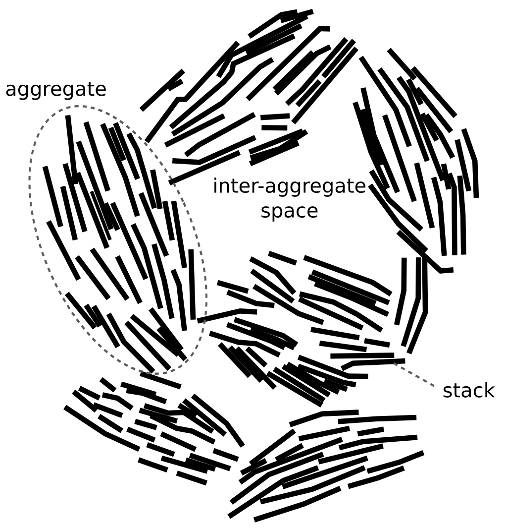
“Schematic particle arrangement in highly compacted Na-bentonite” from Navarro et al. (2017)

Here it is clear that they differ between “aggregates” (which I’m not sure is the same thing as “particles”), “stacks”, and individual TOT-layers (which I assume are represented by the line-shaped objects). In the following, however, we will use the term “stack” to refer to any kind of suggested fundamental structure built up from individual TOT-layers.

The one-sentence version of this blog post is:

Stacks make no sense as fundamental building blocks in models of water saturated, compacted bentonite.

The easiest argument against stacks is, in my mind, to simply work out the geometrical consequences. But before doing that we will examine some of the references given to support statements about stacks in compacted systems. Often, no references are given at all, but when they are, they usually turn out to be largely irrelevant for the system under study, or even to support an opposite view.

Inadequate referencing

As an example (of many) of inadequate referencing, we use the statement above from Churakov et al. (2014) as a starting point. I think this is a “good” statement, in the sense that it makes rather precise claims about how compacted bentonite is supposed to be structured, and provides references for some key statements, which makes it easier to criticize.

Churakov et al. (2014) reference Segad et al. (2010) for the statement that montmorillonite forms “particles” with 5 – 20 TOT-layers. In turn, Segad et al. (2010) write:

Clay is normally not a homogeneous lamellar material. It might be better described as a disordered structure of stacks of platelets, sometimes called tactoids — a tactoid typically consists of 5-20 platelets.19-21

Here the terminology is quite different from the previous quotations: TOT-layers are called “platelets”, and “particles” are called “tactoids”. Still, they use the phrase “stacks of platelets”, so I think we can continue with using “stack” as a sort of common term for what is being discussed.1 We may also note that here is used the word “clay”, rather than “montmorillonite” (as does Bacle et al. (2016)), but it is clear from the context of the article that it really is montmorillonite/bentonite that is discussed.

Anyhow, Segad et al. (2010) do not give much direct information on the claim we investigate, but provide three new references. Two2 of these — Banin (1967) and Shalkevich et al. (2007) — are actually studies on montmorillonite suspensions, i.e. as far away as you can get from compacted bentonite in terms of density; the solid mass fraction in these studies is in the range 1 – 4%.

The average distance between individual TOT-layers in this density limit is comparable with, or even larger than, their typical lateral extension (~100 nm). Therefore, much of the behavior of low density montmorillonite depends critically on details of the interaction between layer edges and various other components, and systems in this density limit behave very differently depending on e.g. ionic strength, cation population, preparation protocol, temperature, time, etc. This complex behavior is also connected with the fact that pure Ca-montmorillonite does not form a sol, while the presence of as little as 10 – 20% sodium makes the system sol forming. The behaviors and structures of montmorillonite suspensions, however, say very little about how the TOT-layers are organized in compacted bentonite.

We have thus propagated from a statement in Churakov et al. (2014), and a similar one in Segad et al. (2010), that montmorillonite in general, in “compacted rocks” forms aggregates of 5 – 20 TOT-layers, to studies which essentially concern different types of materials. Moreover, the actual value of “5 – 20 TOT layers” comes from Banin (1967), who writes

Evidence has accumulated showing that when montmorillonite is adsorbed with Ca, stable tactoids, containing 5 to 20 parallel plates, are formed (1). When the mineral is adsorbed with Na, the tactoids are not stable, and the single plates are separated from each other.

This source consequently claims that the single TOT-layers are the fundamental units, i.e. it provides an argument against any stack concept! (It basically states that pure Ca-montmorillonite does not form a sol.) In the same manner, even though Segad et al. (2010) make the above quoted statement in the beginning of the paper, they only conclude that “tactoids” are formed in pure Ca-montmorillonite.

The swelling and sedimentation behavior of Ca-montmorillonite is a very interesting question, that we do not have all the answers to yet. Still, it is basically irrelevant for making statements about the structure in compacted — sodium dominated3 — bentonite.

Churakov et al. (2014) also give two references for the statement that the “interparticle porosity” in montmorillonite is 10 – 30% of the total porosity: Holmboe et al. (2012) and Kozaki et al. (2001). This is a bizarre way of referencing, as these two studies draw incompatible conclusions, and since Holmboe et al. (2012) — which is the more adequately performed study — state that this type of porosity may be absent:

At dry density \(>1.4 \;\mathrm{g/cm^3}\) , the average interparticle porosity for the [natural Na-dominated bentonite and purified Na-montmorillonite] samples used in this study was found to be \(1.5\pm1.5\%\), i.e. \(\le 3\%\) and significantly lower than previously reported in the literature.

Holmboe et al. (2012) address directly the discrepancy with earlier studies, and suggest that these were not properly analyzed

The apparent discrepancy between the basal spacings reported by Kozaki et al. (1998, 2001) using Kunipia-F washed Na-montmorillonite, and by Muurinen et al. (2004), using a Na-montmorillonite originating from Wyoming Bentonite MX-80, and the corresponding average basal spacings of the [Na-montmorillonite originating from Wyoming bentonite MX-80] samples reported in this study may partly be due to water contents and partly to the fact that only apparent \(\mathrm{d_{001}}\) values using Bragg’s law, without any profile fitting, were reported in their studies.

If Kozaki et al. (2001) should be used to support a claim about “interparticle porosity”, it consequently has to be done in opposition to — not in conjunction with — Holmboe et al. (2012). It would then also be appropriate for authors to provide arguments for why they discard the conclusions of Holmboe et al. (2012).4

Stacks in compacted bentonite make no geometrical sense

The literature is full of fancy figures of bentonite structure involving stacks. A typical example is found in Wu et al. (2018), and looks similar to this:

stacks illustration from Wu et al. (2018)

This illustration is part of a figure with the caption “Schematic representation of the different porosities in bentonite and the potential diffusion paths.”5 The regular rectangles in this picture illustrate stacks that each seems to contain five TOT-layers (I assume this throughout). Conveniently, these groups of five layers have the same length within each stack, while the length varies somewhat between stacks. This is a quite common feature in figures like this, but it is also common that all stacks are given the same length.

Another feature this illustration has in common with others is that the particles are ordered: we are always shown edges of the TOT-layers. I guess this is partly because a picture of a bunch of stacks seen from “the top” would be less interesting, but it also emphasizes the problem of representing the third dimension: figures like these are in practice figures of straight lines oriented in 2D, and the viewer is implicitly required to imagine a 3D-version of this two-dimensional representation.

A “realistic” stack picture

But, even as a 2D-representation, these figures are not representative of what an actual configuration of stacks of TOT-layers looks like. Individual TOT-layers have a distinct thickness of about 1 nm, but varies widely in the other two dimensions. Ploehn and Liu (2006) analyzed the size distribution of Na-montmorillonite (“Cloisite Na+”) using atomic force microscopy, and found an average aspect ratio of 180 (square-root of basal area divided by thickness). A representative single “TOT-line” drawn to scale is consequently quite different from what is illustrated in in most stack-pictures, and look like this (click on the figure to see it in full size)

Representative TOT-layer drawn to scale with water films

In this figure, we have added “water layers” on each side of the TOT-layer (light red), with the water-to-solid volume ratio of 16. Neatly stacking five such units shows that the rectangles in the Wu et al. (2018)-figure should be transformed like this

actual veiw of stacks in Wu et al. (2018)

But this is still not representative of what an assemblage of five randomly picked TOT-layers would look like, because the size distribution has a substantial variance. According to Ploehn and Liu (2006), the aspect ratio follows approximately a log-normal distribution. If we draw five values from this distribution for the length of five “TOT-lines”, and form assemblages, we end up with structures that look like this:7

Five realistic stacks

These are the kind of units that should fill the bentonite illustrations. They are quite irregularly shaped and are certainly not identical (this would be even more pronounced when considering the third dimension, and if the stacks contain more layers).

It is easy to see that it is impossible to construct a dense structure with these building blocks, if they are allowed a random orientation. The resulting structure rather looks something like this

percolation gel with realistic stacks

Such a structure evidently has very low density, and are reminiscent of the gel structures suggested in e.g. Shalkevich et al. (2007) (see fig. 7 in that paper). This makes some sense, since the idea of stacks of TOT-layers (“tactoids”) originated from studies of low density structures, as discussed above.

Note that the structure in pictures like that in Wu et al. (2018) has a substantial density only because it is constructed with stacks with an unrealistic shape. But even in these types of pictures is the density not very high: with some rudimentary image analysis we conclude that the density in the above picture is only around 800 kg/m3. Also the figure from Navarro et al. (2017) above gives a density below 1000 kg/m3, although there it is explicitly stated that it is a representation of “highly compacted bentonite”.

The only manner in which the “realistic” building blocks can be made to form a dense structure is to keep them in the same orientation. The resulting structures then look e.g. like this

Dense structrue of color coded realistic stacks

where we have color coded each stack, to remind ourselves that these units are supposed to be fundamental.

Just looking at this structure of a “stack of stacks” should make it clear how flawed the idea is of stacks as fundamental structural units in compacted bentonite (note also how unrepresentative the stack-pictures found in the literature are). One of many questions that immediately arises is e.g. why on earth the tiny gaps between stacks (indicated by arrows) should remain. This brings us to the next argument against stacks as fundamental units for compacted water saturated bentonite:

What is supposed to keep stacks together?

The pressure configuration in the structure suggested by Navarro et al. (2017)

Assuming that this system is in equilibrium with an external water reservoir at zero pressure (i.e. atmospheric absolute pressure), the pressure in the compartment labeled “intra-aggregate space” is also close to zero. On the other hand, in the “stacks” located just a few nm away, the pressure is certainly above 10 MPa in many places! A structure like this is obviously not in mechanical equilibrium! (To use the term “obvious” here feels like such an understatement.)

Implications

To sum up what we have discussed so far, the following picture emerges. The bentonite literature is packed with descriptions of compacted water saturated bentonite as built up of stacks as fundamental units. These descriptions are so commonplace that they often are not supported by references. But when they are, it seems that the entire notion is based on misconceptions. In particular, structures identified in low density systems (suspensions, gels) have been carried over, without reflection, to descriptions of compacted bentonite. Moreover, all figures illustrating the stack concept are based on inadequate representations of what an arbitrary assemblage of TOT-layers arranged in this way actually would look like. With a “realistic” representation it quickly becomes obvious that it makes little sense to base a fundamental unit in compacted systems on the stack concept.

My impression is that this flawed stack concept underlies the entire contemporary mainstream view of compacted bentonite, as e.g. expressed by Wu et al. (2018):

A widely accepted view is that the total porosity of bentonite consists of \(\epsilon_ {ip}\) and \(\epsilon_ {il}\) (Tachi and Yotsuji, 2014; Tournassat and Appelo, 2011; Van Loon et al., 2007). \(\epsilon_ {ip}\) is a porosity related to the space between the bentonite particles and/or between the other grains of minerals present in bentonite. It can further be subdivided into \(\epsilon_ {ddl}\) and \(\epsilon_ {free}\). The diffuse double layer, which forms in the transition zone from the mineral surface to the free water space, contains water, cations and a minor amount of anions. The charge at the negative outer surface of the montmorillonite is neutralized by an excess of cations. The free water space contains a charge-balanced aqueous solution of cations and anions. \(\epsilon_ {il}\) represents the space between TOT-layers in montmorillonite particles exhibiting negatively charged surfaces. Due to anion exclusion effect, anions are excluded from the interlayer space, but water and cations are present.

This view can be summarized as:

  • The fundamental building blocks are stacks of TOT-layers (“particles”, “aggregates”, “tactoids”, “grains”…)
  • Electric double layers are present only on external surfaces of the stacks.
  • Far away from external surfaces — in the “inter-particle” or “inter-aggregate” pores — the diffuse layers merge with a bulk water solution
  • Interlayer pores are defined as being internal to the stacks, and are postulated to be fundamentally different from the external diffuse layers; they play by a different set of rules.

I don’t understand how authors can get away with promoting this conceptual view without supplying reasonable arguments for all of its assumptions8 — and with such a complex structure, there are a lot of assumptions.

As already discussed, the geometrical implications of the suggested structure do not hold up to scrutiny. Likewise, there are many arguments against the presence of substantial amounts of bulk water in compacted bentonite, including the pressure consideration above. But let’s also take a look at what is stated about “interlayers” and how these are distinguished from electric double layers (I will use quotation marks in the following, and write “interlayers” when specifically referring to pores defined as internal to stacks).

“Interlayers”

“Interlayers” are often postulated to be completely devoid of anions. We discussed this assumption in more depth in a previous blog post, where we discovered that the only references supplied when making this postulate are based on the Poisson-Boltzmann equation. But this is inadequate, since the Poisson-Boltzmann equation does describe diffuse layers, and predicts anions everywhere.

By requiring anion-free “interlayers”, authors actually claim that the physico-chemistry of “interlayers” is somehow qualitatively different from that of “external surfaces”, although these compartments have the exact same constitution (charged TOT-layer surface + ions + water). But an explanation for why this should be the case is never provided, nor is any argument given for why diffuse layer concepts are not supposed to apply to “interlayers”.9 This issue becomes even more absurd given the strong empirical evidence for that anions actually do reside in interlayers.

The treatment of anions is not the only ad hoc description of “interlayers”. It also seems close to mandatory to describe them as having a maximum extension, and as having an extension independently parameterized by sample density. E.g. the influential models for Na-bentonite of Bourg et al. (2006) and Tournassat and Appelo (2011) both rely on the idea that “interlayers” swell out to a certain volume that is smaller than the total pore volume, but that still depends on density.

In e.g. Bourg et al. (2006), the fraction of “interlayer” pores remains essentially constant at ~78%, as density decreases from 1.57 g/cm3 to 1.27 g/cm3, while the “interlayers” transform from having 2 monolayers of water (2WL) to having 3 monolayers (3WL). This is a very strange behavior: “interlayers” are acknowledged as having a swelling potential (2WL expands to 3WL), but do, for some reason, not affect 22% of the pore volume! Although such a behavior strongly deviates from what we expect if “interlayers” are treated with conventional diffuse layer concepts, no mechanism is provided.

In contrast, it should be noted that the established explanation for “tactoid” formation in pure Ca-montmorillonite involves no ad hoc assumptions of this sort, but rests on treating all ions as part of diffuse layers.

Another type of macabre consequence of defining “interlayer” pores as internal to stacks is that a completely homogeneous system is described has having no interlayer pores (because it has no stacks). E.g. Tournassat and Appelo (2011) write (\(n_c\) is the number of TOT-layers in a stack)

[…] the number of stacks in the \(c\)-direction has considerable influence on the interlayer porosity, with interlayer porosity increasing with \(n_c\) and reaching the maximum when \(n_c \approx 25\). The interlayer porosity halves with \(n_c\) when \(n_c\) is smaller than 3, and becomes zero for \(n_c = 1\).10

It is not acceptable that using the term interlayer should require accepting stacks as fundamental units. But the usage of the term as being internal to stacks is so widespread in the contemporary bentonite literature, that I fear it is difficult to even communicate this issue. Nevertheless, I am certain that e.g. Norrish (1954) does not depend on the existence of stacks when using the term like this:

Fig. 7 shows the relationship between interlayer spacing and water content for Na-montmorillonite. There is good agreement between the experimental points and the theoretical line, showing that interlayer swelling accounts for all, or almost all, of physical swelling.

The stack view obstructs real discovery

A severe consequence of the conceptual view just discussed is that “stacking number” — the (average) number of TOT-layers that stacks are supposed to contain — has been established as fitting parameter in models that are clearly over-parameterized. An example of this is Tournassat and Appelo (2011), who write11

Our predictive model excludes anions from the interlayer space and relates the interlayer porosity to the ionic strength and the montmorillonite bulk dry density. This presentation offers a good fit for measured anion accessible porosities in bentonites over a wide range of conditions and is also in agreement with microscopic observations.

But since anions do reside in interlayers,12 it would be better if the model didn’t fit: an over-parameterized or conceptually flawed model that fits data provides very little useful information.

A similar more recent example is Wu et al. (2018). In this work, a model based on the stack concept is successfully fitted both to data on \(\mathrm{ReO_4^-}\) diffusion in “GMZ” bentonite and to data on \(\mathrm{Cl^-}\) diffusion in “KWK” bentonite, by varying “stacking number” (among other parameters). Again, as the model assumes anion-free “interlayer” pores, a better outcome would be if it was not able to fit the data. Moreover, this paper focuses mainly on the ability of the model, while not at all emphasizing the fact that about ten (!) times more \(\mathrm{ReO_4^-}\) was measured in “GMZ” as compared with \(\mathrm{Cl^-}\) in “KWK”, at similar conditions in certain cases. The latter observation is quite puzzling and is, in my opinion, certainly worth deeper investigation (and I am fully convinced that it is not explained by differences in “stacking number”).

Footnotes

[1] The terminology in the bentonite literature is really all over the place. You may e.g. also find the term “tactoid” used as Navarro et al. (2017) use “aggregate”, or the term “platelet” used for a stack of TOT-layers

[2] The third reference is an entire book on clays.

[3] Note that “sodium dominated” in this context means ~20% or more.

[4] It may be noticed that Kozaki et al. (2001) see no X-ray diffraction peaks for low density samples:

The basal spacing of water-saturated montmorillonite was determined by the XRD method. […] It was found that a basal spacing of 1.88 nm, corresponding to the three-water layer hydrate state […] was not observed before the dry density reached 1.0 Mg/m3.

My interpretation of this observation is that the diffraction peak has shifted to even lower reflection angles (in agreement with the observations of Holmboe et al. (2012)), not registered by the equipment. The alternative interpretation must otherwise be that “stacks” suddenly cease to exist below 1.0 g/cm3. (Yet, Kozaki et al. (2001) continues to use a certain d-value in their analysis, also for densities below 1.0 g/cm3.)

[5] I have discussed “diffusion paths” in an earlier blog post. This illustration certainly fits that discussion.

[6] A water-to-solid volume ratio of 1 corresponds basically to interlayers of three monolayers of water (3WL).

[7] To construct these units, I made the additional choice of placing each layer randomly in the horizontal direction, with the constraint that all layers should be confined within the range of the longest one in each unit.

[8] By “get away with” I mean “pass peer-review”, and by “don’t understand” I mean “understand”.

[9] This is reminiscent of how certain authors imply that the interlayer is non-diffusive under so-called crystalline swelling.

[10] A mathematical remark: if the interlayer porosity “halves with \(n_c\)” (what does that mean?) when \(n_c = 2\) (“smaller than 3”), it is impossible to simultaneously have zero interlayer porosity for \(n_c = 1\) (unless the interlayer porosity is zero for any \(n_c\)).

[11] I guess the word “presentation” here really should be “representation”?

[12] Note that one of the authors of this paper also claims in a later paper that anions do populate 3-waterlayer interlayers, in accordance with the Poisson-Boltzmann equation:

The agreement between PB calculations and MD simulation predictions was somewhat worse in the case of the \(\mathrm{Cl^-}\) concentration profiles than in the case of the \(\mathrm{Na^+}\) profiles (Figure 3), perhaps reflecting the poorer statistics for interlayer Cl concentrations […] Nevertheless, reasonable quantitative agreement was found (Table 2).

Swelling pressure, part V: Suction

There are several “descriptions” of bentonite swelling. While a few of them actually denies any significant role played by the exchangeable cations, most of these descriptions treat the exchangeable ions as part of an osmotic system. I have earlier discussed how the terms “osmotic” or “osmosis” may cause some confusion in different contexts, and discussed the confusion surrounding the treatment of electrostatic forces.

In this blog post I discuss the description of bentonite swelling often adopted in the fields of soil mechanics and geotechnical engineering. In particular, we focus on the concept of suction, which is central in these research fields, while being basically absent in others.

As far as I understand, suction is just the water chemical potential “disguised” as a pressure variable; although I have trouble finding clear-cut definitions, it seems clear that suction is directly inherited from the “water potential” concept, which has been central in soil science for a long time. Applied to bentonite, the geotechnical description is thus not principally different from the osmotic approach that I have presented previously. But the way the suction concept is (and isn’t) applied may cause unnecessary confusion regarding the swelling mechanisms. I think a root for this confusion is that suction involves both osmotic and capillary mechanisms.

Matric suction (capillary suction)

Matric suction is typically associated with capillarity, a fundamental mechanism in many conventional soil materials under so-called unsaturated conditions. A conventional soil with a significant amount of small enough pores shows capillary condensation, i.e. it contains liquid water below the condensation point for ordinary bulk water. Naturally, the equilibrium vapor pressure increases with the amount of water in the soil, as the pores containing liquid water become larger. For conventional soils, it therefore makes sense to speak of the degree of saturation of a sample, and to relate saturation and equilibrium vapor pressure by means of a water retention curve. Underlying this picture is the notion that the solid parts constitute a “soil skeleton” (the matrix), and that the soil can be viewed as a vessel that can be more or less filled with water.

The pressure of the capillary water is lower than that of the surrounding air, and is related to the curvature of the interfaces between the two phases (menisci), as expressed by the Young-Laplace equation. For a spherically symmetric meniscus this equation reads

\begin{equation} \Delta p = p_w – p_a = \frac{2\sigma}{r} \tag{1} \end{equation}

where \(p_a\) and \(p_w\) denote the pressures of air and capillary water, respectively, \(\sigma\) is the surface tension, and \(r\) is the radius of curvature of the interface. The sign of \(r\) depends on whether the interface bulges inwards (“concave”, \(r<0\)) or outwards (“convex”, \(r>0\)). For capillary water, \(r\) is negative and \(\Delta p\) — which is also called the Laplace pressure — is a negative quantity.

As far as I understand, matric suction is simply defined as the negative Laplace pressure, i.e.

\begin{equation} s_m = p_a – p_w \tag{2} \end{equation}

With this definition, suction has a straightforward physical meaning as quantifying the difference in pressure of the two fluids occupying the pore space, and clearly relates to the everyday use of the word.

Suction — in this capillary sense — gives a simple principal explanation for (apparent) cohesion in e.g. unsaturated sand: individual grains are pushed together by the air-water pressure difference, as schematically illustrated here (the yellow stuff is supposed to be two grains of sand, and the blue stuff water)

Net force for two sand grains exposed to matric suction

It is reasonable to assume that the net force transmitted by the soil skeleton — usually quantified using the concept of effective stress — governs several mechanical properties of the soil sample, e.g. shear strength. The above description also makes it reasonable to assume that effective stress depends on suction.

Thus, in unsaturated conventional soil are quantities like degree of saturation, pore size distribution, (matric) suction, effective stress, and shear strength very much associated. Another way of saying this is that there is an optimal combination of water content and particle size distribution for constructing the perfect sand castle.

The chemical potential of the capillary water is related to matric suction. Choosing pure bulk water under pressure \(p_a\)1 as reference, the chemical potential of the liquid phase in the soil is obtained by integrating the Gibbs-Duhem equation from \(p_a\) to \(p_w\)

\begin{equation} \mu = \mu_0 + \int_{p_a}^{p_w}v dP = \mu_0 + v\cdot \left(p_w – p_a \right) = \mu_0 -v\cdot s_m \tag{3} \end{equation}

where \(\mu_0\) is the reference chemical potential, \(v\) is the molar volume of water, and we have assumed incompressibility.

The above expression shows that matric suction in this case directly quantifies the (relative) water chemical potential. Note, however, that eq. 3 does not define matric suction; \(s_m\) is defined as a pressure difference between two phases (eq. 2), and happens to quantify the chemical potential under the present circumstances (pure capillary water).

A chemical potential can generally be expressed in terms of activity (\(a\))

\begin{equation} \mu = \mu_0 + RT \ln a \tag{4} \end{equation}

For our case, water activity is to a very good approximation equal to relative humidity, the ratio between the vapor pressures in the state under consideration and in the reference state, i.e. \(a = p_v/p_{v,0}\). Combining eqs. 3 and 4, we see that the vapor pressure in this case is related to matric suction as

\begin{equation} \frac{p_v}{p_{v,0}} = e^{-v\cdot s_m/RT} \end{equation}

Using the Young-Laplace equation (eq. 1) for \(s_m\) we can also write this as

\begin{equation} \frac{p_v}{p_{v,0}} = e^{\frac{2v\sigma}{RTr}} \end{equation}

This is the so-called Kelvin equation, which relates the equilibrium vapor pressure to the curvature of an air-pure water interface. Note that, since \(r<0\) for capillary water, the vapor pressure is lower than the corresponding bulk value (\(p_v < p_{v,0}\)).

Osmotic suction and total suction

So far, we have discussed suction in a capillary context, and related it to water chemical potential or vapor pressure. Now consider how the picture changes if the pores in our conventional soil contain saline water. Matric suction — i.e. the actual pressure difference between the pore solution and the surrounding air, sticking with eq. 2 as the definition — is in general different from the pure water case, because solutes influence surface tension. Also, water activity (vapor pressure) is different from the pure water case, but there is no longer a direct relation between water activity and matric suction, because water activity is independently altered by the presence of solutes.

The water chemical potential of a saline bulk solution (i.e. with no capillary effects), can be written in terms of the osmotic pressure, \(\pi(c)\)

\begin{equation} \mu(c) = \mu_0 – v\cdot\pi(c) \tag{5} \end{equation}

where we have assumed a salt concentration \(c\), and indicated that the osmotic pressure, and hence the chemical potential, depends on this concentration.

Although eq. 5 is of the same form as eq. 3, matric suction and osmotic pressure are very different quantities. The former is defined under circumstances where an actual pressure difference prevail between the air and water phases. In contrast, there is no pressure difference between the phases in a container containing both a solution and a gas phase. \(\pi(c)\) corresponds to the elevated pressure that must be applied for the solution to be in equilibrium with pure water kept at the reference pressure.

Despite the different natures of matric suction and osmotic pressure, the fields of geotechnical engineering and soil mechanics insist on also referring to \(\pi(c)\) as a suction variable: the osmotic suction. Similarly, total suction is defined as the sum of matric and osmotic suction

\begin{equation} \Psi = s_m + \pi(c) \end{equation}

These definitions seem to have no other purpose than to be able to write the water chemical potential generally as

\begin{equation} \mu = \mu_0 -v\cdot \Psi \tag{6} \end{equation}

Total suction is thus de facto defined simply as the (relative) value of the water chemical potential, expressed as a pressure (I think this is completely analogous to “total water potential” in soil science).

Eq. 6 shows that \(\Psi\) is directly related to water activity, or vapor pressure, and we can write

\begin{equation} \frac{p_v}{p_{v,0}} = e^{-v\cdot \Psi/RT} \tag{7} \end{equation}

This relation is quite often erroneously referred to as the Kelvin equation (or “Kelvin’s law”) in the bentonite literature. But note that the above equation just restates the definition of water activity, because \(v\cdot\Psi\) cannot be reduced to anything more concrete than the relative value of the water chemical potential. The Kelvin equation, on the other hand, expresses something more concrete: the equilibrium vapor pressure for a curved air-water interface. Some clay literature refer to the above relation as the “Psychrometric law”, but that name seems not established in other fields.2

A definition is motivated by its usefulness, and total change in water chemical potential is of course central when considering e.g. moisture movement in soil. My non-geotechnical brain, however, is not fond of extending the “suction” variable in the way outlined above. To start with, there is already a variable to use: the water chemical potential. Also, “total suction” no longer has the direct relation to the everyday use of the word suction: there is no “sucking” going on in a saline bulk solution,3 while in a capillary there is. Furthermore, with a saline pore solution there is no direct relation between (total) suction and e.g. effective stress or shear strength.

Although both matric suction and osmotic pressure under certain circumstances can be measured in a direct way, it seems that (total) suction usually is quantified by measuring/controlling the vapor pressure with which the soil sample is in equilibrium. Actually, one of the more comprehensive definitions of various “suctions” that I have been able to find — in Fredlund et al. (2012) — speaks only of various vapor pressures (although based on the capillary and osmotic concepts):4

Matric or capillary component of free energy: Matric suction is the equivalent suction derived from the measurement of the partial pressure of the water vapor in equilibrium with the soil-water relative to the partial pressure of the water vapor in equilibrium with a solution identical in composition with the soil-water.

Osmotic (or solute) component of free energy: Osmotic suction is the equivalent suction derived from the measurement of the partial pressure of the water vapor in equilibrium with a solution identical in composition with the soil-water relative to the partial pressure of water vapor in equilibrium with free pure water.

Total suction or free energy of soil-water: Total suction is the equivalent suction derived from the measurement of the partial pressure of the water vapor in equilibrium with the soil-water relative to the partial pressure of water vapor in equilibrium with free pure water.

It seems that such operational definitions of suction has made the term synonymous with “vapor pressure depression” in large parts of the bentonite scientific literature.

Suction in bentonite

In the above discussion we had mainly a conventional soil in mind. When applying the suction concepts to bentonite,5 I think there are a few additional pitfalls/sources for confusion. Firstly, note that the definitions discussed previously involve “a solution identical in composition with the soil-water”. But soil-water that contains appreciable amounts of exchangeable ions — as is the case for bentonite — cannot be realized as an external solution.

It seems that this “complication” is treated by assuming that an external solution in equilibrium with a bentonite sample is the soil-water (this is analogous to how many geochemists use the term “porewater” in bentonite contexts). Not surprisingly, this treatment has bizarre consequences. The conclusion for e.g. a salt free bentonite sample — which is in equilibrium with pure water — is that it lacks osmotic suction, and that its lowered vapor pressure (when isolated and unloaded) is completely due to matric suction! I think this is such an odd outcome that it is worth repeating: A system dominated by interlayer pores, containing dissolved cations at very high concentrations, is described as lacking osmotic pressure! It is not uncommon to find descriptions like this one (from Lang et al. (2019))

The total suction of unsaturated soils consists of matric and osmotic suctions (Yong and Warkentin, 1975; Fredlund et al., 2012; Lu and Likos, 2004). In clays, the matric suction is due to surface tension, adsorptive forces and osmotic forces (i.e. the diffuse double layer forces), whereas the osmotic suction is due to the presence of dissolved solutes in the pore water.

We apparently live in a world where “matric suction” consists of “osmotic forces”, while the same “osmotic forces” do not contribute to “osmotic suction”. Except when the clay contains excess ions, in which case we have an arbitrary combination of the two “suctions” (note also that “osmotic suction” and “osmotic swelling” are two quite different things).

Although the above consequence is odd, it is still only a matter of definition: accepting that “matric suction” involves osmotic forces (which I don’t recommend), the description may still be adequate in principle; after all, “total suction” quantifies the reduction of the water chemical potential.

But the focus on “matric suction” also reveals a conceptual view of bentonite structure that I find problematic: it suggests a first order approximation of bentonite as a conventional soil, i.e. as an assemblage of solid grains separated from an aqueous phase (and a gas phase). This “matric” view is fully in line with the idea of “free water” in bentonite, and it is quite clear that this is a prevailing view in the geotechnical, as well as in the geochemical, literature. For instance, with the formulation “the presence of dissolved solutes in the pore water” in the above quotation, the “pore water” the authors have in mind is a charge neutral bulk water solution.

With the “matric” conceptual view, the degree of saturation becomes a central variable in much soil mechanical analyses of bentonite. When dealing with actual unsaturated bentonite samples, I guess this makes sense, but once a sample is saturated this variable has lost much of its meaning.6 Consider e.g. the different expected behaviors if drying e.g. a water saturated metal filter or a saturated bentonite sample.

The different nature of drying a metal filter compared with drying a saturated bentonite sample

The equilibrium vapor pressure of both these systems is lower than the corresponding pure bulk water value. For the metal filter, the lowered water activity is of course due to capillarity, i.e. there is an actual pressure reduction in the water phase (matric suction!). When lowering the external vapor pressure below the equilibrium point (i.e. drying), capillary water migrates out of the filter, while the metal structure itself remains intact. In this case, as the system remains defined in a reasonable way, it is motivated to speak of the saturation state of the filter.

For a drying bentonite sample, the behavior is not as well defined, and depends on how the drying is performed and on initial water content. For a quasi-static process, where the external vapor pressure is lowered in small steps at an arbitrary slow rate, it should be clear that the entire sample will respond simply by shrinking. In this case it does not make much sense to speak of the sample as still being saturated, nor to speak of it as having become unsaturated.

For a more “violent” drying process, e.g. placing the bentonite sample in an oven at 105 °C , it is also clear that — rather than resulting in a neatly shrunken, dense piece of clay — the sample now will suffer from macroscopic cracks and other deformations. Neither in this case does it make much sense to try to define the degree of saturation, in relation to the sample initially put in the oven.

Note also that if we, instead of drying, increase the external vapor pressure from the initial equilibrium value, the metal filter will not respond much at all, while the bentonite sample immediately will begin to swell.

I hope that this example has made it clear, not only that the degree of saturation is in general ill-defined for bentonite, but also that a bentonite sample behaves more as an aqueous solution rather than as a conventional soil: if we alter external vapor pressure, an aqueous solution responds by either “swelling” (taking up water) or “shrinking” (giving off water). A main aspect of this conceptual view of bentonite — which we may call the “osmotic” view — is that water does not form a separate phase.7 This was pointed out e.g. by Bolt and Miller (1958) (referring to this type of system as an “ideal clay-water system”)

In contrast to the familiar case described is the ideal clay-water system in which the particles are not in direct contact but are separated by layers of water. Removal of water from such a system does not introduce a third phase but merely causes the particles to move closer to one another with the pores remaining water saturated.

From these considerations it follows that a generally consistent treatment is to relate bentonite water activity to water content, rather than to degree of saturation.

Another consequence of adopting a “matric” view of bentonite (i.e. to include osmotic forces in “matric suction”) is that “matric suction” loses its direct connection with effective stress. This can be illustrated by taking the “osmotic” view: just as the mechanical properties of an aqueous solution (e.g. viscosity) do not depend critically on whether or not it is under (osmotic) pressure, we should not expect e.g. bentonite shear strength to be directly related to swelling pressure.8

Footnotes

[1] Often, the air is at atmospheric pressure, in which case the reference is the ordinary standard state.

[2] The relatively common misspelling “Psychometric law” is kind of funny.

[3] The cautious reader may remark that saline solutions do “suck”, in terms of osmosis. But note the following: 1) Osmosis requires a semi-permeable membrane, separating the solution from an external water source. We have said nothing about the presence of such a component in the present discussion. The way osmotic suction sometimes is described in the literature makes me suspect that some authors are under the impression that the mere presence of a solute causes a pressure reduction in the liquid. 2) In the presence of a semi-permeable membrane, osmosis has no problem occurring without a pressure difference between between the two compartments. 3) For cases when the solution is acted on by an increased hydrostatic pressure, water is transported from lower to higher pressure. It is difficult to say that there is any “sucking” in such a process (I would argue that the establishment of a pressure difference is an effect, rather than a cause, in the case of osmosis) 4) The idea that a solution has a well-defined partial water pressure is wrong.

[4] I’m still not fully satisfied with this definition: It may be noted that the definitions are somewhat circular (“matric suction is the equivalent suction…”), so they still require that we have in mind that “suction” also is defined in terms of a certain vapor pressure ratio (e.g. eq. 7). Note also that the headings speak of “free energy”. Perhaps I am nitpicking, but (free) energy is an extensive quantity, while suction (pressure) is intensive. Thus, “free energy” here really mean “specific free energy” (or “partial free energy”, i.e. chemical potential). I think the soil science literature in general is quite sloppy with making this distinction.

[5] “Bentonite” is used in the following as an abbreviation for bentonite and claystone, or any clay system with significant cation exchange capacity.

[6] If you press bentonite granules to form a cohesive sample you certainly end up with a system having both water filled interlayer pores and air-filled macropores (or perhaps an even more complex pore structure). This blog post mainly concerns saturated bentonite, by which I mean bentonite material which does not contain any gas phase. We can thus speak of saturated bentonite, although a degree of saturation variable is not well defined.

[7] Rather, montmorillonite and water form a homogeneous mixture.

[8] However, bentonite strength relates indirectly to swelling pressure (under specific conditions) because both quantities depends on a third: density.

Sorption part III: Donnan equilibrium in compacted bentonite

Consider this basic experiment: contact a water saturated sample of compacted pure Na-montmorillonite, with dry mass 10 g and cation exchange capacity 1 meq/g, with an external solution of 100 ml 0.1 M KCl. Although such an experiment has never been reported1, I’m convinced that all agree that the outcome would be similar to what is illustrated in this animation.

Hypothetical ion equilibrium test

Potassium diffuses in, and sodium diffuses out of the sample until equilibrium is established. At equilibrium also a minor amount of chloride is found in the sample. The indicated concentration levels are chosen to correspond roughly to results from from similar type of experiments.2

Although results like these are quite unambiguous, the way they are described and modeled in the bentonite3 literature is, in my opinion, quite a mess. You may find one or several of the following terms used to describe the processes

  • Cation exchange
  • Sorption/Desorptioṇ
  • Anion exclusion
  • Accessible porosity
  • Surface complexation
  • Donnan equilibrium
  • Donnan exclusion
  • Donnan porosity/volume
  • Stern layer
  • Electric double layer
  • Diffuse double layer
  • Triple layer
  • Poisson-Boltzmann
  • Gouy-Chapman
  • Ion equilibrium

In this blog post I argue for that the primary mechanism at play is Donnan equilibrium, and that most of the above terms can be interpreted in terms of this type of equilibrium, while some of the others do not apply.

Donnan equilibrium: effect vs. model

In the bentonite literature, the term “Donnan” is quite heavily associated with the modeling of anion equilibrium; e.g. the term “Donnan exclusion” is quite common , and you may find statements that researchers use “Donnan porespace models” as models for “anion exclusion”, or a “Donnan approach” to model “anion porosity”.4 Sometimes the term “Donnan effect” is used synonymously with “Salt exclusion”. Also when authors acknowledge cations as being part of “Donnan” equilibrium, the term is still used mainly to label a model or an “approach”.

But I would like to push for that “Donnan equilibrium” primarily should be the name of an observable effect, and that it applies equally to both anions and cations. This effect — which was hypothesized by Gibbs already in the 1870s — relies basically only on two things:

  • An electrolytic system, i.e. the presence of charged aqueous species (ions).
  • The presence of a semi-permeable component that is permeable to some of the charges, but does not allow for the passage of at least one type of charge.

In equilibrated systems fulfilling these requirements it is — to use Donnan’s own words — “thermodynamically necessary” that the permeant ions distribute unequally across the semi-permeable component. This phenomenon — unequal ion distributions on the different sides of the semi-permeable component — should, in my opinion, be the central meaning of the term “Donnan equilibrium”.

The first publication of Donnan on the effect actually concerned osmotic pressure response, in systems of Congo Red separated from solutions of sodium chloride and sodium hydroxide. The same year (1911) he also published the ionic equilibrium equations for some specific systems.5 In particular he considered the equilibrium of NaCl initially separated from NaR, where R is an impermeant anion (e.g. that of Congo Red), leading to the famous relation (“int” denotes the solution containing R)

\begin{equation} c_\mathrm{Na^+}^\mathrm{ext}\cdot c_\mathrm{Cl^-}^\mathrm{ext} = c_\mathrm{Na^+}^\mathrm{int}\cdot c_\mathrm{Cl^-}^\mathrm{int} \tag{1} \end{equation}

Unfortunately, this relation alone (or relations derived from it) is often what the term “Donnan” is associated with in today’s clay research literature, with the implication that systems not obeying it are not Donnan systems. But the above relation assumes ideal conditions and complete ionization of the salts — issues Donnan persistently seems to have grappled with. In a review on the effect he writes

The exact equations can, however, be stated only in terms of the chemical potentials of Willard Gibbs, or of the ion activities or ionic activity-coefficients of G. N. Lewis. Indeed an accurate experimental study of the equilibria produced by ionically semi-permeable membranes may prove to be of value in the investigation of ionic activity coefficients.

It must therefore be understood that, if in the following pages ionic concentrations and not ionic activities are used, this is done in order to present a simple, though only approximate, statement of the fundamental relationships.

The issue of (the degree of) ionization was explicitly addressed in publications following the 1911 article; Donnan & Allmand (1914) motivated their investigations of the \(\mathrm{KCl/K_4Fe(CN)_6}\) system by that “it was deemed advisable to test the relation when using a better defined, non-dialysable anion than that of Congo-red”, and the study of the Na/K equilibrium in Donnan & Garner (1919) used ferrocyanide solutions on both sides of the membrane in an attempt to overcome the difficulty of the “uncertainty as to the manner of ionisation of potassium ferrocyanide” (and thus for the simplified equations to apply).

I mean that since non-ideality and ion association are general issues when treating salt solutions, it does not make much sense to use the term “Donnan equilibrium” only when some particular equation applies; as long as the mechanism for the observed behavior is that some charges diffuse through a semi-permeable component, while some others don’t, the effect should be termed Donnan equilibrium.

Donnan equilibrium in gels, soils and clays

After Donnan’s original publications in 1911, the effect was soon recognized in colloidal systems. Procter & Wilson (1916) used Donnan’s equations to analyze the swelling of gelatin jelly immersed in hydrochloric acid. In this case chloride is the charge compensating ion, allowed to move between the phases, while the immobile charge is positive charges on the gelatin network. Thus, no semi-permeable membrane is necessary for the effect; alternatively one could say that the gel constitutes its own semi-permeable component. The Donnan equilibrium in protein solutions was further and extensively investigated by Loeb.

As far as I am aware, Mattson was first to identify the Donnan effect in “soil” suspensions,6 attributing e.g. “negative adsorption” of chloride as a consequence of Donnan equilibrium, and explicitly referencing the works of Procter and Loeb. Mattson describes the suspension in terms of electric double layers with a diffuse “atmosphere of cations” surrounding the “micelle” (the soil particle), and refers to Donnan equilibrium as the distribution of an electrolyte between the “micellar” and the “inter-micellar” solutions. Oddly,7 he uses Donnan’s original framework (e.g. eq. 1) to quantify the equilibrium, although the electrostatic potential and the ion concentrations varies significantly in the investigated systems. A more appropriate treatment would thus be to use e.g. the Gouy-Chapman description for the ion distribution near a charged plane surface (which he refers to!).

Instead, Schofield (1947) analyzed Mattson’s data using this approach. He also comments on its (the Gouy-Chapman model) range of validity

… [T]he equation is applicable to cases in which the distance between opposing surfaces considerably exceeds the distance between neighboring point charges on the surfaces; for there will then be a range of electrolyte concentrations over which the radius of the ionic atmosphere is less than the former and greater than the latter. In Mattson’s measurements on bentonite suspension, these distances are roughly 500 A. and 10 A. respectively, so there is an ample margin.

He continues to comment on the validity of Donnan’s original equations

When the distance ratio has narrowed to unity, it is to be expected that the system will conform to the equation of the Donnan membrane equilibrium. This equation fits closely the measurements of Procter on gelatine swollen in dilute hydrochloric acid. […] In a bentonite suspension the charges are so far from being evenly distributed that the Donnan equation is not even approximately obeyed.

From these statements it should be clear that the general behavior (cation exchange, salt exclusion) of ions in bentonite equilibrated with an external solution is due to the Donnan effect.8 The appropriate theoretical treatment of this effect differs, however, depending on details of the investigated system. To argue whether or not e.g. the Gouy-Chapman description should be classified as a “Donnan” approach is purely semantic.

It is also clear that in the case of compacted bentonite the distance ratio is narrowed to unity — the typical interlayer distance is 1 nm, which also is the typical distance between structural charges in the montmorillonite particles. It is thus expected that Donnan’s original treatment may work for such systems (adjusted for non-ideality), while the Gouy-Chapman description is not valid.9

The message I am trying to convey is neatly presented in Overbeek (1956) — a text I highly recommend for further information. Overbeek distinguishes between “classical” (Donnan’s original) and “new” (accounting for variations in potential etc.) treatments of Donnan equilibrium, and says the following about dense systems

If the particles come very close together the potential drop between [surface and interlayer midpoint] becomes smaller and smaller as illustrated in Fig. 4. This means that the local concentrations of ions are not very variable and that we are again back at the classical Donnan situation, where distribution of ions, osmotic pressure and Donnan potential are simply given by the elementary equations as treated in section 2. It is remarkable that the new treatment of the Donnan effects may deviate strongly from the classical treatment when the colloid concentration is low, but not when it is high.

It thus seems plausible that Donnan equilibrium in compacted bentonite can be treated using Donnan’s original equations. But — as interlayer pores are a quite extreme chemical environment — substantial non-ideal behavior may be expected. Treating such behavior is a large challenge for chemical modeling of compacted bentonite, but can not be avoided, since interlayers dominate the pore structure.

Cation exchange is Donnan equilibration

The term “Donnan” in modern bentonite literature is, as mentioned, quite heavily associated with the fate of anions interacting with bentonite. In contrast, cations are often described as being “sorbed” onto the “solids”. This sorption is usually separated into two categories: cation exchange and surface complexation.

Surface complexation reactions are typically described using “surface sites”, and are usually written something like this (exemplified with sodium sorption)

\begin{equation} \equiv \mathrm{S^-} + \mathrm{Na^{+}(aq)} \leftrightarrow \equiv \mathrm{SNa} \end{equation}

where the “surface site” is labeled \(\equiv \mathrm{S}^-\)

Cation exchange is also typically written in terms of “sites”, but requires the exchange of ions (duh!), like this (here exemplified for calcium/sodium exchange)

\begin{equation} \mathrm{2XNa} + \mathrm{Ca^{2+}(aq)} \leftrightarrow \mathrm{X_2Ca} + 2\mathrm{Na^+(aq)} \tag{2} \end{equation}

where X represents an “exchange site” in the solid phase.

In the clay literature the distinction between “surface complexation” and “ion exchange” reactions is rather blurred. You can e.g. find statements that “the ion exchange model can be seen as a limiting case of the surface complex model…”, and it is not uncommon that ion exchange is modeled by means of a surface complexation model. It also seems rather common that ion exchange is understood to involve surface complexation.

Underlying these modeling approaches and descriptions is the (sometimes implicit) idea that exchanged ions are immobile, which clearly has motivated e.g. the traditional diffusion-sorption model for bentonite and claystone. This model assumes that ion exchange binds cations to the solid, making them immobile, while diffusion occurs solely in a bulk water phase (which, incredibly, is assumed to fill the entire pore volume).

However, the idea that the exchanged ion is immobile does not agree with descriptions in the more general ion exchange literature, which instead acknowledge the process as an aspect of the Donnan effect.

Indeed, already in 1919, Donnan & Garner reported Na/K exchange equilibrium in a system consisting of two ferrocyanide solutions separated by a membrane impermeable to ferrocyanide, and it is fully clear that the particular distribution of cations in such systems is just as “thermodynamically necessary” as the distribution of chloride in the initial work on Congo Red and ferrocyanide.

Applied to clays, it is clear that cation exchange occurs even without postulating specific “sorption sites” or immobilization. On the contrary, ion exchange occurs in Donnan systems precisely because the ions are mobile.

In his book “Ion exchange”,10 Freidrich Helfferich describes ion exchange as diffusion, and distinguishes it from “chemical” processes

Occasionally, ion exchange has been referred to as a “chemical” process, in contrast to adsorption as a “physical” process. This distinction, though plausible at first glance, is misleading. Usually, in ion exchange as a redistribution of ions by diffusion, chemical factors are less significant than in adsorption where the solute is held by the sorbent by forces which may not be purely electrostatic.

Furthermore, in describing a general ion exchange system, he states the exact characteristics of a Donnan system, with the crucial point that the exchangeable ion is “free”, albeit subject to the constraint of electroneutrality

Ion exchangers owe their characteristic properties to a peculiar feature of their structure. They consist of a framework which is held together by chemical bonds or lattice energy. This framework carries a positive or negative electric surplus charge which is compensated by ions of opposite sign, the so-called counter ions. The counter ions are free to move within the framework and can be replaced by other ions of the same sign. The framework of a cation exchanger may be regarded as a macromolecular or crystalline polyanion, that of an anion exchanger as a polycation.

To give a very simple picture, the ion exchanger may be compared to a sponge with counter ions floating in the pores. When the sponge is immersed in a solution, the counter ions can leave the pores and float out. However, electroneutrality must be preserved, i.e., the electric surplus charge of the sponge must be compensated at any time by a stoichiometrically equivalent number of counter ions within the pores. Hence a counter ion can leave the sponge only when, simultaneously, another counter ion enters and takes over the task of contributing its share to the compensation of the framework charge.

With this “sponge” model at hand, he argues for that the reaction presented in eq. 2 above should be reformulated

[T]he model shows that ion exchange is essentially a statistical redistribution of counter ions between the pore liquid and the external solution, a process in which neither the framework nor the co-ions take part. Therefore Eqs. (1-1) [eq. 2 above] and (1-2) should be rewritten: \begin{equation} 2\overline{\mathrm{Na^+}} + \mathrm{Ca^{2+}} \leftrightarrow \overline{\mathrm{Ca^{2+}}} + 2\mathrm{Na^{+}} \end{equation} \begin{equation} 2\overline{\mathrm{Cl^-}} + \mathrm{SO_4^{2+}} \leftrightarrow \overline{\mathrm{SO_4^{2-}}} + 2\mathrm{Cl^{-}} \end{equation} Quantities with bars refer to the inside of the ion exchanger.

This “statistical redistribution” is of course nothing but the establishment of Donnan equilibrium between the external solution and the exchanger phase (as in the animation above). Naturally, Donnan equilibrium — using either the “classical” or the “new” equations — is at the heart of many analyses of ion exchange systems.

Unfortunately, this has not been the tradition in the compacted bentonite research field, where a “diffuse layer” approach to cation exchange has only been considered in more recent years, and then usually as a supplement to already existing models and tools. We are therefore in the rather uneasy situation that ion exchange in bentonite nowadays often is explained in terms of both a Donnan effect and as specific surface complexation.

Considering the robust evidence for significant ion mobility in interlayer pores, I strongly doubt surface complexation to be relevant for describing ion exchange in bentonite.11 Instead, I believe that not separating these processes obscures the analysis of species that actually do sorb in these systems. In any event, the exact effects of Donnan equilibrium — a mechanism dependent on nothing but that some charges diffuses through the semi-permeable component, while some others don’t — must first and foremost be worked out.

A demonstration of compacted bentonite as a Donnan system

To demonstrate how well the Donnan effect in compacted bentonite is captured by Donnan’s original description, we use the following relation, derived from eq. 1 (i.e we assume only the presence of a 1:1 salt, apart from the impermeable component)

\begin{equation} \frac{c_\mathrm{Cl^-}^\mathrm{int}}{c_\mathrm{Cl^-}^\mathrm{ext}} = -\frac{1}{2}\frac{z}{c_\mathrm{Cl^-}^\mathrm{ext}} + \sqrt{\frac{1}{4} (\frac{z}{c_\mathrm{Cl^-}^\mathrm{ext}})^2+1} \tag{3} \end{equation}

Here \(z\) denotes the concentration of cations compensating impermeable charge. Eq. 3 quantifies anion exclusion, and is seen to depend only on the ratio \(c_\mathrm{Cl^-}^\mathrm{ext}/z\).

This equation is plotted in the diagram below, together with data of chloride exclusion in sodium dominated bentonite (Van Loon et al., 2007) and in potassium ferrocyanide (Donnan & Allmand, 1914)

Anion exclusion in bentonite and ferrocyanide compared with Donnan's ideal formula

I find this plot amazing. Although some points refer to bentonite at density 1900 \(\mathrm{kg/m^3}\) (corresponding to \(z \approx 5\) M), while others refer to a solution of approximately 25 mM \(\mathrm{K_4Fe(CN)_6}\) (\(z \approx 0.1\) M), the anion exclusion behavior is basically identical! Moreover, it fits the ideal “Donnan model” (eq. 3) quite well!

There is of course a lot more to be said about the detailed behavior of these systems, but I think a few things stand out:

  • It should be obvious that the basic mechanism for anion exclusion is the same in these two systems. This observed similarity thus invalidates the idea that anion exclusion in compacted bentonite is due to an intricate, ionic strength-dependent partitioning of a complex pore structure into parts which either are, or are not, accessible to chloride. In other words, the above plot is another demonstration that the concept of “accessible anion porosity” is nonsense.
  • The similarity between compacted bentonite and the simpler ferrocyanide system confirms Overbeek’s statement above, that Donnan’s “elementary” equations apply when the colloid concentration (i.e. density) is high enough.
  • The slope of the curve at small external concentrations directly reflects the amount of exchangeable cations that contributes to the Donnan effect. The similarity between model and experimental data thus confirms that the major part of the cations are mobile, i.e. not adsorbed by surface complexation. The similarity between the bentonite system and the ferrocyanide system also suggests that non-ideal corrections to the theory is better dealt with by means of e.g. activity coefficients, rather than by singling out a quite different mechanism (surface complexation) in one of the systems.

Footnotes

[1] The only equilibrium study of this kind I am aware of, that involves compacted, purified, homo-ionic clay, is Karnland et al. (2011). This study concerns Na/Ca exchange, and does not investigate the associated chloride equilibrium.

[2] I have assumed a K/Na selectivity coefficient of 2, and 95% salt exclusion.

[3] “Bentonite” is used in the following as an abbreviation for bentonite and claystone, or any clay system with significant cation exchange capacity.

[4] This particular publication states that I am one of the researchers using a “Donnan approach” to model “anion porosity”. Let me state for the record that I never have modeled “anion porosity”, or have any intentions to do so.

[5] This article has an English translation.

[6] In my head, a “soil suspension” and a “soil particle” are not very well defined entities. As I understand, Mattson investigated “Sharkey soil” and “Bentonite”. Sharkey soil is reported to have a cation exchange capacity of around 0.3 eq/kg, and the bentonite appear to be of “Wyoming” type. It is thus reasonably clear that Mattson’s “soil” particles are montmorillonite particles.

[7] Mattson and co-workers published a whole series of papers on “The laws of soil colloidal behavior” during the course of over 15 years, and appear to have caused both awe and confusion in the soil science community. I find it a bit amusing that there is a published paper (Kelley, 1943) which in turn reviews and comments on Mattson’s papers. Some statements in this paper include: “It seems to be generally agreed that some of [Mattsons papers] are difficult to understand.” and “The extensive use by [Mattson and co-workers] of terms either coined by them or used in new settings, the frequent contradictions of statement and inconsistencies in definition, and perhaps most important of all, the use by the authors of theoretical reasoning founded, not on experimentally determined data, but on calculations based on purely hypothetical premises, make it difficult to condense these papers into a form suitable for publication without doing injustice to the authors or sacrificing strict accuracy.

[8] It may be worth noting that the only works referenced by Schofield — apart from a paper on dye adsorption — are Mattson, Procter and Donnan. Remarkably, Gouy is not referenced!

[9] Of course, one can instead solve the Poisson-Boltzmann equation for “overlapping” double layers.

[10] In its introduction is found the following gem: “A spectacular evolution began in 1935 with the discovery by two English chemists, Adams and Holmes, that crushed phonograph records exhibit ion-exchange properties.” Who wouldn’t want to hear more of that story?!

[11] As a further argument for that the concept of immobile exchangeable ions in bentonite is flawed, one can take a look at the spread in reported values for the fraction of such ions. You can basically find any value between \(>99\%\) and \(\sim 0\%\) for the same type of systems. To me, this indicates overparameterization rather than physical significance.

Sorption part II: Letting go of the bulk water

Disclaimer: The following discussion applies fully to ions that only interact with bentonite by means of being part of an electric double layer. Here such ions are called “simple” ions. Species with more specific chemical interactions will be discussed in separate blog posts.

The “surface diffusion” model is not suitable for compacted bentonite

In the previous post on sorption1 we derived a correct “surface diffusion” model. The equation describing the concentration evolution in such a model is a real Fick’s second law, meaning that it only contains the actual diffusion coefficient (apart from the concentration itself)

\begin{equation}
\frac{\partial c}{\partial t} = D_\mathrm{sd} \cdot\nabla^2 c \tag{1}
\end{equation}

Note that \(c\) in this equation still denotes the concentration in the presumed bulk water,2 while \(D_\mathrm{sd}\) relates to the mobility, on the macroscopic scale, of a diffusing species in a system consisting of both bulk water and surfaces.3

Conceptually, eq. 1 states that there is no sorption in a surface diffusion model, in the sense that species do not get immobilized. Still, the concept of sorption is frequently used in the context of surface diffusion, giving rise to phrases such as “How Mobile Are Sorbed Cations in Clays and Clay Rocks?”. The term “sorption” has evidently shifted from referring to an immobilization process, to only mean the uptake of species from a bulk water domain to some other domain (where the species may or may not be mobile). In turn, the role of the parameter \(K_d\) is completely shifted: in the traditional model it quantifies retardation of the diffusive flux, while in a surface diffusion model it quantifies enhancement of the flux (in a certain sense).

A correct4 surface diffusion model resolves several of the inconsistencies experienced when applying the traditional diffusion-sorption model to cation diffusion in bentonite. In particular, the parameter referred to as \(D_e\) may grow indefinitely without violating physics (because it is no longer a real diffusion coefficient), and the insensitivity of \(D_\mathrm{sd}\) to \(K_d\) may be understood because \(D_\mathrm{sd}\) is the real diffusion coefficient (it is not an “apparent” diffusivity, which is expected to be influenced by a varying amount of immobilization).

Still, a surface diffusion model is not a very satisfying description of bentonite, because it assumes the entire pore volume to be bulk water. To me, it seems absurd to base a bentonite model on bulk water, as the most characteristic phenomenon in this material — swelling — relies on it not being in equilibrium with a bulk water solution (at the same pressure). It is also understood that the “surfaces” in a surface diffusion model correspond to montmorillonite interlayer spaces — here defined as the regions where the exchangeable ions reside5 — which are known to dominate the pore volume in any relevant system.

Indeed, assuming that diffusion occurs both in bulk water and on surfaces, it is expected that \(D_\mathrm{sd}\) actually should vary significantly with background concentration, because a diffusing ion is then assumed to spend considerably different times in the two domains, depending on the value of \(K_d\).6

Using the sodium diffusion data from Tachi and Yotsuji (2014) as an example, \(\rho\cdot K_d\) varies from \(\sim 70\) to \(\sim 1\), when the background concentration (NaCl) is varied from 0.01 M to 0.5 M (at constant dry density \(\rho=800\;\mathrm{kg/m^3}\)). Interpreting this in terms of a surface diffusion model, a tracer is supposed to spend about 1% of the time in the bulk water phase when the background concentration is 0.01 M, and about 41% of the time there when the background concentration is 0.5 M7. But the evaluated values of \(D_\mathrm{sd}\) (referred to as “\(D_a\)” in Tachi and Yotsuji (2014)) show a variation less than a factor 2 over the same background concentration range.

Insignificant dependence of \(D_\mathrm{sd}\) on background concentration is found generally in the literature data, as seen here (data sources: 1, 2, 3, 4, 5)

Diffusion coefficients as a function of background concentration for Sr, Cs, and Na.

These plots show the deviation from the average of the macroscopically observed diffusion coefficients (\(D_\mathrm{macr.}\)). These diffusion coefficients are most often reported and interpreted as “\(D_a\)”, but it should be clear from the above discussion that they equally well can be interpreted as \(D_\mathrm{sd}\). The plots thus show the variation of \(D_\mathrm{sd}\), in test series where \(D_\mathrm{sd}\) (reported as “\(D_a\)”) has been evaluated as a function of background concentration.8 The variation is seen to be small in all cases, and the data show no systematic dependencies on e.g. type of ion or density (i.e., at this level of accuracy, the variation is to be regarded as scatter).

The fact that \(D_\mathrm{sd}\) basically is independent of background concentration strongly suggests that diffusion only occurs in a single domain, which by necessity must be interlayer pores. This conclusion is also fully in line with the basic observation that interlayer pores dominate in any relevant system.

Diffusion in the homogeneous mixture model

A more conceptually satisfying basis for describing compacted bentonite is thus a model that assigns all pore volume to the surface regions and discards the bulk water domain. I call this the homogeneous mixture model. In its simplest version, diffusive fluxes in the homogeneous mixture model is described by the familiar Fickian expression

\begin{equation} j = -\phi\cdot D_c \cdot \nabla c^\mathrm{int} \tag{2} \end{equation}

where the concentration of the species under consideration, \(c^\mathrm{int}\), is indexed with an “int”, to remind us that it refers to the concentration in interlayer pores. The corresponding diffusion coefficient is labeled \(D_c\). Notice that \(c^\mathrm{int}\) and \(D_c\) refer to macroscopic, averaged quantities; consequently, \(D_c\) should be associated with the empirical quantity \(D_\mathrm{macr.}\) (i.e. what we interpreted as \(D_\mathrm{sd}\) in the previous section, and what many unfortunately interpret as \(D_a\)) — \(D_c\) is not the short scale diffusivity within an interlayer.

For species that only “interact” with the bentonite by means of being part of an electric double layer (“simple” ions), diffusion is the only process that alters concentration, and the continuity equation has the simplest possible form

\begin{equation} \frac{\partial n}{\partial t} + \nabla\cdot j = 0 \end{equation}

Here \(n\) is the total amount of diffusing species per volume porous system, i.e. \(n = \phi c^\mathrm{int}\). Inserting the expression for the flux in the continuity equation we get

\begin{equation} \frac{\partial c^\mathrm{int}}{\partial t} = D_c \cdot \nabla^2 c^\mathrm{int} \tag{3} \end{equation}

Eqs. 2 and 3 describe diffusion, at the Fickian level, in the homogeneous mixture model for “simple” ions. They are identical in form to the Fickian description in a conventional porous system; the only “exotic” aspect of the present description is that it applies to interlayer concentrations (\(c^\mathrm{int}\)), and more work is needed in order to apply it to cases involving external solutions.

But for isolated systems, e.g. closed-cell diffusion tests, eq. 3 can be applied directly. It is also clear that it will reproduce the results of such tests, as the concentration evolution is known to obey an equation of this form (Fick’s second law).

Model comparison

We have now considered three different models — the traditional diffusion-sorption model, the (correct) surface diffusion model, and the homogeneous mixture model — which all can be fitted to closed-cell diffusion data, as exemplified here

three models fitted to diffusion data for Sr from Sato et al. (92)

The experimental data in this plot (from Sato et al. (1992)) represent the typical behavior of simple ions in compacted bentonite. The plot shows the resulting concentration profile in a Na-montmorillonite sample of density 600 \(\mathrm{kg/m^3}\), where an initial planar source of strontium, embedded in the middle of the sample, has diffused for 7 days. Also plotted are the identical results from fitting the three models to the data (the diffusion coefficient and the concentration at 0 mm were used as fitting parameters in all three models).

From the successful fitting of all the models it is clear that bentonite diffusion data alone does not provide much information for discriminating between concepts — any model which provides a governing equation of the form of Fick’s second law will fit the data. Instead, let us describe what a successful fit of each model implies conceptually

  • The traditional diffusion-sorption model

    The entire pore volume is filled with bulk water, in contradiction with the observation that bentonite is dominated by interlayer pores. In the bulk water strontium diffuse at an unphysically high rate. The evolution of the total ion concentration is retarded because most ions sorb onto surface regions (which have zero volume) where they become immobilized.

  • The “surface diffusion” model

    The entire pore volume is filled with bulk water, in contradiction with the observation that bentonite is dominated by interlayer pores. In the bulk water strontium diffuse at a reasonable rate. Most of the strontium, however, is distributed in the surface regions (which have zero volume), where it also diffuse. The overall diffusivity is a complex function of the diffusivities in each separate domain (bulk and surface), and of how the ion distributes between these domains.

  • The homogeneous mixture model

    The entire pore volume consists of interlayers, in line with the observation that bentonite is dominated by such pores. In the interlayers strontium diffuse at a reasonable rate.

From these descriptions it should be obvious that the homogeneous mixture model is the more reasonable one — it is both compatible with simple observations of the pore structure and mathematically considerably less complex as compared with the others.

The following table summarizes the mathematical complexity of the models (\(D_p\), \(D_s\) and \(D_c\) denote single domain diffusivities, \(\rho\) is dry density, and \(\phi\) porosity)

Summary models

Note that the simplicity of the homogeneous mixture model is achieved by disregarding any bulk water phase: only with bulk water absent is it possible to describe experimental data as pure diffusion in a single domain. This process — pure diffusion in a single domain — is also suggested by the observed insensitivity of diffusivity to background concentration.

These results imply that “sorption” is not a valid concept for simple cations in compacted bentonite, regardless of whether this is supposed to be an immobilization mechanism, or if it is supposed to be a mechanism for uptake of ions from a bulk water to a surface domain. For these types of ions, closed-cell tests measure real (not “apparent”) diffusion coefficients, which should be interpreted as interlayer pore diffusivities (\(D_c\)).

Footnotes

[1] Well, the subject was rather on “sorption” (with quotes), the point being that “sorbed” ions are not immobilized.

[2] Eq. 1 can be transformed to an equation for the “total” concentration by multiplying both sides by \(\left (\phi + \rho\cdot K_d\right)\).

[3] Unfortunately, I called this quantity \(D_\mathrm{macr.}\) in the previous post. As I here compare several different diffusion models, it is important to separate between model parameters and empirical parameters, and the diffusion coefficient in the “surface diffusion” model will henceforth be called \(D_\mathrm{sd}\). \(D_\mathrm{macr.}\) is used to label the empirically observed diffusion parameter. Since the “surface diffusion” model can be successfully fitted to experimental diffusion data, the value of the two parameters will, in the end, be the same. This doesn’t mean that the distinction between the parameters is unimportant. On the contrary, failing to separate between \(D_\mathrm{macr.}\) and the model parameter \(D_\mathrm{a}\) has led large parts of the bentonite research community to assume \(D_\mathrm{a}\) is a measured quantity.

[4] It might seem silly to point out that the model should be “correct”, but the model which actually is referred to as the surface diffusion model in the literature is incorrect, because it assumes that diffusive fluxes in different domains can be added.

[5] There is a common alternative, implicit, and absurd definition of interlayer, based on the stack view, which I intend to discuss in a future blog post. Update (220906): This interlayer definition and stacks are discussed here.

[6] Note that, although \(D_\mathrm{sd}\) is not given simply by a weighted sum of individual domain diffusivities in the surface diffusion model, it is some crazy function of the ion mobilities in the two domains.

[7] With this interpretation, the fraction of bulk water ions is given by \(\frac{\phi}{\phi+\rho K_d}\).

[8] The plot may give the impression that such data is vast, but these are basically all studies found in the bentonite literature, where background concentration has been varied systematically. Several of these use “raw” bentonite (“MX-80”), which contains soluble minerals. Therefore, unless this complication is identified and dealt with (which it isn’t), the background concentration may not reflect the internal chemistry of the samples, i.e. the sample and the external solution may not be in full chemical equilibrium. Also, a majority of the studies concern through-diffusion, where filters are known to interfere at low ionic strength, and consequently increase the uncertainty of the evaluated parameters. The “optimal” tests for investigating the behavior of \(D_\mathrm{macr.}\) with varying background concentrations are closed-cell tests on purified montmorillonite. There are only two such tests reported (Kozaki et al. (2008) and Tachi and Yotsuji (2014)), and both are performed on quite low density samples.

Bentonite swelling pressure, part IV: electrostatics

Swelling is not due to electrostatic repulsion between montmorillonite particles

Few things confuse me more than how the role of electrostatics in clay swelling is described in the scientific literature. Consider e.g. this statement from Bratko et al. (1986)

The interaction between charged aggregates in solution is generally interpreted in terms of electrostatic repulsion between double layers surrounding the aggregates.

But in the same paper we learn that the main contribution to the force between two charged surfaces in solution is the entropy of mixing of counter-ions, and that electrostatic interactions actually may result in an attractive force between the surfaces.

Nevertheless, I think Bratko et al. (1986) are right: swelling is, for some reason, often “interpreted” in terms of electrostatic repulsion between electric double layers. It is easy to find statements that e.g. the expression for the osmotic pressure in the Gouy-Chapman model describes “the electrostatic force per unit area”, or that lamellar phases are “electrostatically swollen”, with an osmotic pressure “mainly of electrostatic origin”. Segad (2013) writes

The interactions between the negatively charged platelets lead to a repulsive long-ranged electrostatic force promoting swelling.

and Tester et al. (2016) write

The DLVO theory describes the interaction between two colloidal particles as a balance between electrostatic repulsion, in this case between two negatively charged clay layers, and vdW attraction.

Laird (2006) claims that electrostatics cause both repulsion and (strong) attraction between clay layers

A balance between strong electrostatic-attraction and hydration-repulsion forces controls crystalline swelling. The extent of crystalline swelling decreases with increasing layer charge. Double-layer swelling occurs between quasicrystals. An electrostatic repulsion force develops when the positively charged diffuse portions of double layers from two quasicrystals overlap in an aqueous suspension. Layer charge has little or no direct effect on double-layer swelling.

Although many authors reasonably understand the actual mechanisms of double layer repulsion, I think it is very unfortunate that this language is established and contributes to unnecessary confusion.

To gain some intuition for that clay swelling is not primarily due to electrostatic repulsion between montmorillonite particles, let us consider the Poisson-Boltzmann equation. This is, after all, the description usually referred to when authors speak of “electrostatic repulsion” between clay layers. The Poisson-Boltzmann equation may be used to describe the electrostatic potential, and the corresponding counter-ion equilibrium distribution, between two equally charged surfaces, and a typical result looks like this1

Solution Poisson-Boltzmann

Here we assume two negatively charged parallel surfaces with uniform charge density, and the counter-ions are represented by a continuous charge density. The system is assumed infinitely extended in the x- (in/out of the page) and y- (up/down) directions, and thus rotationally symmetric around the z-axis.

With a lot of equal charges “facing” each other, the illustration may indeed give the impression that there somehow is an electrostatic repulsion between the surfaces. That this is not the case, however, may be seen from the symmetry of the potential. In fact, replacing one of the negatively charged surfaces by a neutral surface at half the distance does not change the solution to the Poisson-Boltzmann equation! A charged and a neutral surface thus experience the same repulsion as two charged surfaces, if only placed at half the distance.2

charged-neutral and charged-chared diffuse layer

With one surface being uncharged, “interpreting” the force as an electrostatic repulsion between the particles makes little sense.

A related way to convince yourself that there is no electrostatic repulsion between the two charged surfaces is to consider the electric field generated by one “half” of the original system. This field vanishes on the outside of the considered “half”-system.

E-field vanishes outside "half"-system

This means that removing a “half”-system would not be “noticed” by the other “half”-system, in the sense that the electric field configuration remains the same (and corresponds to having a neutral particle at half the distance).

It may be helpful to also remember from electrostatics that the electric field outside a plate capacitor vanishes. Thus, configuring two plate capacitors as shown below, there is no electric field between the positively charged surfaces, regardless of how close they are.3

Two plate capacitors

This “plate capacitor” configuration is actually reminiscent of the charge distribution in an interlayer at low water content (where the continuum assumption of the Poisson-Boltzmann equation is not valid).

A squeezed ion cloud

Having established that there is no direct electrostatic repulsion between clay particles, the obvious question is: what is the main cause for the repulsion? What the two configurations above have in common — with either two charged surfaces or one charged and one neutral surface — is that they restrict the counter ions to a certain volume. Hence, there is an entropic driving force for transporting more water into the region between the surfaces, thereby pushing them apart. Nelson (2013) describes this quite well4

One may be tempted to say, “Obviously two negatively charged surfaces will repel.” But wait: Each surface, together with its counterion cloud, is an electrically neutral object! Indeed, if we could turn off thermal motion the mobile ions would collapse down to the surfaces, rendering them neutral. Thus the repulsion between like-charged surfaces can only arise as an entropic effect. As the surfaces get closer than twice their Gouy–Chapman length, their diffuse counterion clouds get squeezed; they then resist with an osmotic pressure.

Notice that the presence of this osmotic pressure requires contact with an “external” solution. The existence of a repulsive force between clay layers thus requires that water is available to be transported into the interlayer region. This seems to often be “forgotten” about in many descriptions of clay swelling. But let Kjellander et al. (1988) remind us

The PB pressure between two planar surfaces with equal surface charge equals \(P_\mathrm{ionic} = k_BT\sum_i n_i(0)\), where \(n_i(0)\) is the ion density at the midplane between the surfaces. Due to symmetry there is no electrostatic force between the two halves of the system (the electrostatic fluctuation forces due to ion-ion correlations are neglected). To obtain the net pressure when the system is surrounded by a bulk electrolyte solution, it is necessary to subtract the external pressure calculated in the same approximation; this is given by the ideal gas contribution \(P_\mathrm{bulk} = k_BT \sum_i n_i^\mathrm{bulk}\).

There is no repulsive force of this kind in an isolated, internally equilibrated, clay.

Moreover, the force is usually conceived of as repulsive because the water chemical potential of the surrounding (“external”) solution is typically larger than in the clay. But from an osmotic viewpoint there is nothing fundamentally different going on when the external phase is, say, vapor of low pressure (set e.g. by a saturated salt solution), causing the clay to lose water, i.e to shrink. Thus, if swelling is “interpreted” as electrostatic repulsion between montmorillonite particles, then drying should be “interpreted” as electrostatic attraction between the same particles.

The fact that there is repulsion — in the osmotic sense — between a montmorillonite particle and a neutral surface has huge implications for how to handle interfaces between montmorillonite and other phases in compacted bentonite components. Rather than to simply assume these to contain bulk water (“free water”), there is every reason to believe that the physico-chemical conditions at such interfaces are similar to “ordinary” interlayer pores. Since any type of mineral alteration occurs at such interfaces, there is no escape from understanding interlayer chemistry if a satisfying geochemical description of bentonite is desired.

The role of electrostatics in clay swelling

Although swelling is not primarily due to direct electrostatic repulsion between clay particles, electrostatics is of course essential to consider when calculating the osmotic pressure. And rather than contributing to repulsion, electrostatic interactions actually reduce the pressure. This is clearly seen from e.g. the Poisson-Boltzmann solution for two charged surfaces, where the resulting osmotic pressure corresponds to an ideal solution with a concentration corresponding to the value at the midpoint (cf. the quotation from Kjellander et al. (1988) above). But the midpoint concentration — and hence the osmotic pressure — is lowered as compared with the average, because of electrostatic attraction between layers and counter-ions.

Midpoint concentration reduces

Moreover, a treatment of the electrostatic problem beyond the mean-field (i.e. beyond the Poisson-Boltzmann description) shows that ion-ion correlation cause an explicit attraction between equally charged surfaces (similar to a van der Waals force). In systems with divalent counter ions, this attraction is large enough to prevent swelling beyond a certain limit — a prediction in qualitative agreement with observation. Electrostatics could thus be claimed to contribute to prevent clay swelling.

I think comparison with a simple salt solution can be useful. Nobody (?) would come up with the idea that the primary reason for the osmotic pressure of a NaCl solution is due to electrostatic repulsion between, say, chloride ions. In fact, the electrostatic interactions in such a solution reduce the osmotic pressure compared with a corresponding ideal solution.

Below is plotted the swelling pressure of Na-montmorillonite as a function of the average concentration of counter-ions (data from here). For comparison, the osmotic pressures of a NaCl solution and an ideal solution are also plotted (data from here), as a function of the total amount of ions (i.e. two times the NaCl concentration)5

Osmotic pressure Na-mmt and NaCl

This plot demonstrates the attractive aspect of electrostatic interactions in these systems. While the NaCl pressure is only slightly reduced, Na-montmorillonite shows strong non-ideal behavior. In the “low” concentration regime (\(<2\) mol/kgw) we understand the pressure reduction as an effect of counter-ions electrostatically attracted to the clay surfaces. The dramatic increase of swelling pressure in the high concentration limit is reasonably an effect of hydration of ions and surfaces; it should be kept in mind that an average ion concentration of 3 mol/kgw in Na-montmorillonite roughly corresponds to a water-to-solid-mass ratio of only 0.3, and an average interlayer width below 1 nm.

Even though there seems to be quite some confusion regarding clay swelling pressure in the bentonite literature, the message here is not that everything about it is in reality understood. On the contrary, there are quite a number of behaviors that, as far as I’m aware, lack fully satisfactory explanations. For example, at room temperature the basal spacing in Ca-montmorillonite is never observed to be larger than \(\sim 19\) Å6, corresponding to a (dry) density of approximately \(1300 \;\mathrm{kg/m^3}\); yet, this material systematically exerts swelling pressure at considerably lower density (\(\sim 700 \;\mathrm{kg/m^3}\)). But in order to tackle issues like these, it is essential to be clear about the swelling mechanisms that we actually do understand.

Update (221018): A correction to this blog post is discussed here.

Footnotes

[1] This particular calculation uses the formulas presented in Engström and Wennerström (1978), and assumes mono-valent counter-ions at room temperature, a charge density of \(-0.1 \;\mathrm{C/m^2}\), and a surface-surface distance of 2 nm.

[2] Here is only considered the Poisson-Boltzmann pressure. If e.g. van der Waals attraction between the surfaces is included, the resulting forces are not necessarily equal. The point here, however, concerns the repulsion due to the presence of diffuse layers.

[3] Having strictly zero field is of course an ideal result, corresponding to an infinitely extended capacitor.

[4] The quotation is taken from a draft version of this book.

[5] The graph denoted “Ideal solution” is simply the van’t Hoff relation \(\Pi = RT c\), which strictly is only valid in the low concentration limit. It is nevertheless here extended to the whole concentration range. In the same way, the NaCl-curve is simply \(\Pi = \varphi RT c\), where \(\varphi\) is the osmotic coefficient for NaCl. Sorry about that.

[6] Upon cooling, Svensson and Hansen (2010) actually observed a basal spacing of 21.6 Å in pure Ca-montmorillonite.

Filter influence: why cation through-diffusion tests at low ionic strength should be avoided

In through-diffusion tests, diffusion is monitored from an external source reservoir, through a clay sample, into an external target reservoir. As the sample typically is sandwiched between two confining filters, the full set-up can be abstracted as transport across three conductive components, coupled in series (filter-clay-filter).

Solving this problem — which is not specifically related to diffusion in clay, and applies equally well to e.g. electric currents or laminar fluid flow — the steady-state flux can be written as (for details, see appendix)

\begin{equation} j = D_\mathrm{e}^\mathrm{clay}\frac{1}{1+\omega} \frac{c_\mathrm{source}}{L_\mathrm{clay}} \tag{1} \end{equation}

where \(\omega\) is the relative filter resistance

\begin{equation} \omega =D_\mathrm{e}^\mathrm{clay}\left (\frac{1}{D_\mathrm{e}^\mathrm{filter1}} + \frac{1}{D_\mathrm{e}^\mathrm{filter2}} \right ) \frac{L_\mathrm{filter}}{L_\mathrm{clay}} \tag{2} \end{equation}

Here \(D_e\) denotes the effective diffusivity for the different components1, \(c_\mathrm{source}\) is the constant source reservoir concentration, \(L_\mathrm{clay}\) is the length of the clay sample, and \(L_\mathrm{filter}\) is the length of the filters (we assume that the two filters have the same length).

Eq. 1 shows that in the limit \(\omega \ll 1\), the flux is expressed solely in terms of clay parameters2

\begin{equation} j = D_\mathrm{e}^\mathrm{clay}\cdot \frac{c_\mathrm{source}} {L_\mathrm{clay}} \end{equation}

In the other limit (\(\omega \gg 1\)), the flux is instead completely controlled by the filters,

\begin{equation} j = \frac{D_\mathrm{e}^\mathrm{filter1} \cdot D_\mathrm{e}^\mathrm{filter2}} { D_\mathrm{e}^\mathrm{filter1}+D_\mathrm{e}^\mathrm{filter2}} \cdot \frac{c_\mathrm{source}}{L_\mathrm{filter}} \end{equation}

i.e. independent of any clay parameters.

It is thus clear that through-diffusion tests should be designed to have \(\omega\) reasonably small; preferably, one should have \(\omega \ll 1\), which allows for leaving the filters out of the analysis.

While filter parameters in practice are limited to a quite small range for a given ion3, \(D_\mathrm{e}^\mathrm{clay}\) is known to grow indefinitely for many cations, as the background concentration tends to zero1. Consequently, for such ions, there always exists a background concentration limit, beyond which the filters completely control the resulting flux (i.e. where \(\omega \gg 1\)).

Even though the effect of filters in through-diffusion tests has been identified for a
long time
, there are numerous examples in the bentonite literature where filter influence is ignored, or not fully identified, leading to erroneous interpretations. For example, when describing through-diffusion tests with strontium in Boom Clay, Altmann et al. (2012) write

The resulting \(\alpha\) value of \(\sim 440\) corresponds to a \(K_d\) value similar to that measured on dispersed and intact Boom Clay. However, if this \(\alpha\) is used to estimate the corresponding \(D_e\) value via \(D_e = \alpha\cdot D_a\), the value obtained is \(\sim 45\) times higher than \(D_e(\mathrm{HTO})\), which is an unrealistically large difference. This is probably because the necessary conditions for calculating \(D_e\) by Fick’s law were not satisfied as indicated by the fact that the concentration profiles measured at the end of the through-diffusion experiment were unexpectedly ‘flat’, i.e. did not vary in a linear fashion between the surfaces in contact with the source and sink solutions. The reason for this behaviour is not yet known.

But a “flat” concentration profile is a key signature of filters limiting the flux, as the (external) concentration difference across the clay is (see appendix)

\begin{equation} c_\mathrm{in} – c_\mathrm{out} = \frac{c_\mathrm{source}}{1+\omega} \end{equation}

which approaches zero when \(\omega\) becomes large.

Consequently, the reported behavior strongly indicates that Boom Clay has a very high transport capacity for strontium under the right conditions (the test was performed with a sodium background concentration of approximately 0.02 M), leading to the filters limiting the flux. This, in turn, implies that the value for \(D_e\) in the clay is underestimated, rather than being “unrealistically large”.

What is demonstrated in this test — but not concluded — is that the principal diffusion mechanism in Boom Clay is the same as in compacted bentonite: ions assumed “sorbed” contribute to — and probably dominate — the diffusive flux. The traditional sorption-diffusion model is not valid for Boom Clay.

Glaus et al. (2007) clearly demonstrate filter influence on Na diffusion in Na-montmorillonite, performed over a large range of \(\mathrm{NaClO_4}\) background concentrations. The concentration profiles across the samples at the time of termination look like this4

Sodium tracer profiles from Glaus et al. (2007)

The profiles become increasingly “flat” with decreasing background concentration, demonstrating an increasing transport capacity of the clay (demonstrating this transport capacity was the main purpose of the study). The tests in Glaus et al. (2007) are analyzed assuming a filter-clay-filter configuration, with identical diffusivities for the two filters (for a given test). The clay component is described using the traditional sorption-diffusion model5. From the reported fitted model parameters, we can calculate the corresponding relative filter resistances, using eq. 2. The result is as follows (all these samples have \(L_\mathrm{clay}=5.4\) mm and \(L_\mathrm{filter}=1.55\) mm.)

\(C_\mathrm{bkg}\)(\(\mathrm{mol/m^3}\)) 10 100 500 700 1000
Reported
\(D_\mathrm{e}^\mathrm{clay}\)(\(10^{-10}\;\mathrm{m^2/s}\))143.70.860.530.38
\(D_\mathrm{e}^\mathrm{filter}\)(\(10^{-10}\;\mathrm{m^2/s}\))0.861.00.860.860.86
Calculated
\(\omega\)(-)9.32.10.60.40.3

Indeed, \(\omega \gg 1\) for the test performed at 10 mM \(\mathrm{NaClO_4}\), and filters fully control the flux. Filter influence is also significant in the test at 100 mM (\(\omega = 2.1\)), while the effect is less important in the tests at higher background concentration. These results fully reflect the appearance of the concentration profiles above.

The filter influence is also clearly seen in the behavior of the outfluxes at the different background concentrations (dotted graphs)

sodium tracer outflux and source concentration evolution in Glaus et al. (2007)

For the tests at high background concentration (i.e. small \(\omega\)), steady-state6 is reached in about 8 – 10 days. In the 10 mM-test, on the other hand, the system is far from steady-state even after 45 days7 — the outflux is still increasing, even though the source concentration (dash-dotted graphs) has dropped significantly. A prolonged transient state is thus another key signature of filters limiting the flux.

This prolonged transient appears because the clay has to be “filled up” with ions before a steady-state can be established. It is important not to confuse this effect with that of retardation due to increased “sorption”: here, it is the filters that cannot “fill up” the clay fast enough, while the diffusive transport capacity of the clay actually increases with increasing “sorption”. Note that this increased transport capacity is not due to increased diffusivity, but exactly because the clay accommodates an increasing amount of tracers as the background concentration decreases.

For the most part, Glaus et al. (2007) treat the filter influence adequately, allowing them to draw correct conclusions regarding diffusion in compacted bentonite. Going into detail, however, I think there is some inconsistency in the parameters, demonstrating the inherent difficulties with handling cation through-diffusion at low ionic strength. \(K_d\) has, as far as I see, been used as a free fitting parameter in the modeling of the tests.8 But for the specific case of sodium tracers diffusing in pure sodium montmorillonite, this parameter is constrained by the simple relation (which also is derived in the article)

\begin{equation} K_d = \frac{\mathrm{CEC}} {1\;\mathrm{eq/mol}} \cdot \frac{1} {C_\mathrm{bkg}} \tag{3} \end{equation}

where \(C_{bkg}\) denotes the background concentration, and CEC is the cation exchange capacity. The reported \(K_d\) values, thus corresponds to these CEC values

\(C_\mathrm{bkg}\)(\(\mathrm{mol/m^3}\)) 10 100 500 700 1000
Reported
\(K_d\)(\(10^{-3}\) \(\mathrm{m^3/kg}\))467.31.81.20.74
Calculated
CEC(eq/kg)0.460.730.900.840.74

As the documented CEC for the used material (purified “Milos” montmorillonite) is \(\sim 0.88\) eq/kg, this evaluation indicates that the fitted \(K_d\) is significantly underestimated for the test performed at 10 mM.

The reason for this underestimation can be further investigated by using the end values of the recorded clay concentration profile, and assuming the CEC value (i.e. assuming \(K_d\), using eq. 3). From the definition of \(K_d\) we can thereby calculate \(c_\mathrm{in}\) and \(c_\mathrm{out}\).

\(C_\mathrm{bkg}\)(\(\mathrm{mol/m^3}\)) 10 100 500 700 1000
Reported
\(s_{in}\)(\(10^{-12}\) mol/kg)88.538.512.29.37.8
\(s_{out}\)(\(10^{-12}\) mol/kg)76.317.41.41.1\(\sim 0\)
\(c_{source}\)(\(10^{-9}\) \(\mathrm{mol/m^3}\))3.110.58.17.79.4
Assumed
\(K_d\)(\(10^{-3}\) \(\mathrm{m^3/kg}\))888.81.761.260.88
Calculated
\(c_{in}\)(\(10^{-9}\) \(\mathrm{mol/m^3}\))1.04.46.97.48.9
\(c_{out}\)(\(10^{-9}\) \(\mathrm{mol/m^3}\))0.92.00.80.9\(\sim 0\)
\(\omega\)(-)21.363.370.310.19\(\sim 0\)

This calculation gives a concentration drop across the inlet filter (\(c_\mathrm{source} – c_\mathrm{in}\)) that is considerably larger than half the value of the concentration in the source reservoir (\(c_\mathrm{source}\)), for the tests made at 10 mM and 100 mM. Such a behavior is impossible if the diffusivities of the two filters are identical! This reevaluation thus suggests that it is not strictly valid to assume identical filter diffusivities when evaluating these kinds of tests. Of course, if the tests are performed under conditions with small \(\omega\), this assumption will make little difference, because the filter influence is anyway small. But under conditions with \(\omega \gg 1\), the exact values of both filter diffusivities will significantly influence the analysis. The concentration profiles across the filters in the 10 mM case can be illustrated like this

concentration profile across fileters, assuming symmetric or assymetric configurations

The main achievement in Glaus et al. (2007) is that they, despite filter transport complications, manage to verify that the effective diffusivity in the clay, both for sodium and strontium tracers, scale with sodium background concentration as

\begin{equation} D_\mathrm{e}^\mathrm{clay} \propto \frac{1}{C_\mathrm{bkg}^Z} \tag{4} \end{equation}

where \(Z\) is the valency of the tracer (i.e., \(Z = 1\) for sodium, and \(Z = 2\) for strontium). Not only is this relation crucial for understanding bentonite diffusion at a deeper level, it also allows for assessing filter influence on evaluated diffusion parameters in general. Eq. 4 implies a dramatic effect of the background concentration on the relative filter resistance for strontium (note from eq. 2 that also \(\omega\) will scale as \(C_\mathrm{bkg}^{-Z}\)): lowering the background concentration e.g. from 0.5 M to 0.1 M, increases \(\omega\) by a factor of 25; lowering it from 0.5 M to 0.01 M gives a factor of 2500! (I don’t think it is a coincidence that the strontium tests in Glaus et al. (2007) are restricted to \(C_\mathrm{bkg}\ge 0.5\;\mathrm{M}\).)

Molera and Eriksen (2002) report diffusion parameters evaluated for strontium in “MX-80” bentonite of various densities and in the background concentration (\(\mathrm{NaClO_4}\)) range 0.5 M – 0.01 M. The tests were evaluated using the traditional sorption-diffusion model for the clay, and by taking the filters into account. The filter diffusivities were, however, assumed identical in the two filters, and kept constant (for a given ion) in all models. From the reported fitted parameters, we can evaluate \(\omega\), using eq. 2 (they used “\(D_\mathrm{a}\)” as fitting parameter rather than \(D_\mathrm{e}^\mathrm{clay}\), but these are related via \(D_\mathrm{e}^\mathrm{clay} = D_\mathrm{a}\left(\phi + \rho K_d\right)\))

ReportedCalculated
Density\(C_\mathrm{bkg}\)\(D_\mathrm{a}\)\(K_d\)\(D_\mathrm{e}^\mathrm{clay}\)\(\omega\)
(\(\mathrm{kg/m^3}\))(\(\mathrm{mol/m^3}\))(\(10^{-10}\;\mathrm{m^2/s}\))(\(10^{-3}\;\mathrm{m^3/kg}\))(\(10^{-10}\;\mathrm{m^2/s}\))(-)
4001000.4311019.36.8
8001000.3515042.214.8
8005000.40155.11.8
1200100.2150012644.2
12001000.1813028.29.9
12005000.25134.01.4
1600100.14120026994.2
16001000.109014.45.1
16005000.20154.91.7
18001000.098013.04.6
18005000.12153.31.1

In this evaluation is used \(D_\mathrm{e}^\mathrm{filter} = 0.925 \cdot 10^{-10}\;\mathrm{m^2/s}\), \(L_\mathrm{filter} = 0.81\) mm, and \(L_\mathrm{clay} = 5.0\) mm for all tests.

Filter transport dominates (\(\omega \gg 1\)) in all but the tests performed at 500 mM (and even in these tests, there is significant filter influence). It can therefore be questioned whether the parameters have been adequately evaluated. That the fitted parameter values (\(K_d\) and/or \(D_\mathrm{a}\)) are not adequate is seen when plotting \(D_\mathrm{e}^\mathrm{clay}\) against background concentration (the “expected dependency” line assumes the \(D_\mathrm{e}^\mathrm{clay}\) value of the 1200 \(\mathrm{kg/m^3}\) sample at 500 mM background concentration).

Effective diffusivities for strontium in Molera and Eriksen (2002)

The \(D_\mathrm{e}^\mathrm{clay}\) values do not obey Glaus’ relation, which they are expected to do, as “MX-80” is a sodium dominated clay. Note that the above plot suggests that \(D_\mathrm{e}^\mathrm{clay}\) in Molera and Eriksen (2002) at background 0.01 M may be underestimated by roughly two orders of magnitude! Nevertheless, the actual clay diffusivity estimated in this study (unfortunately interpreted as “apparent” diffusivity) compares relatively well with other measurements, e.g. Kim et al. (1993), indicating that the underestimation of \(D_\mathrm{e}^\mathrm{clay}\) is rooted in a similar underestimation of \(K_d\).

Results like those of Glaus et al. (2007) and Molera and Eriksen (2002) show that cation through-diffusion tests at low background concentration should be avoided if possible: Both studies explicitly take into account filters when evaluating model parameters, yet the evaluations can be demonstrated to be inconsistent in the low background concentration limit. Although experimental design — as well as corresponding modeling — can be of various quality, the low concentration limit is fundamental: no matter how rigorous the analysis, the results will still be uncertain, simply because the experiment itself conveys less and less information on transport parameters in the clay.

Thus, unless the explicit purpose is to explore the low background concentration limit, it is better to stay away from it, thereby reducing the risk of drawing incorrect conclusions. An example of using data influenced by filter resistance to draw far-reaching conclusions regarding bentonite structure is found in Tinnacher et al. (2016).

This study uses the result from a single through-diffusion test in pure Na-montmorillonite (prepared from SWy-2) at 800 \(\mathrm{kg/m^3}\)9 to review “single porosity models”, and to argue for that this system is dominated by bulk water (\(>70\%\)) — a rather bizarre conclusion, in my opinion.

The test was done with a background electrolyte of 0.1 M NaCl, by adding a small amount of \(\mathrm{CaBr_2}\) (1 mM) to the source reservoir, and monitoring the accumulation of calcium and bromide in the target reservoir (which was kept virtually tracer free by frequent replacement). The recorded normalized outflux of calcium looks like this10

calcium outflux in Tinnacher et al. (2016)

As this test concerns diffusion of a di-valent cation at relatively low ionic strength, there are strong reasons to suspect that filter resistance influences the flux evolution. If I understand correctly, this test was actually performed using the exact same equipment as used in the study by Molera and Eriksen (2002), where we evaluated a value \(\omega = 14.8\) for strontium at the same conditions, albeit in a different clay material (see above).

But using the reported model parameters in Tinnacher et al. (2016) gives \(\omega = 0.77\) (\(D_\mathrm{e}^\mathrm{clay} = 2.06\cdot 10^{-10}\; \mathrm{m^2/s}\), \(D_\mathrm{e}^\mathrm{filter} = 0.85\cdot 10^{-10}\; \mathrm{m^2/s}\), \(L_\mathrm{filter} = 0.79\) mm, and \(L_\mathrm{clay} = 5\) mm). This result — indicating only moderate filter influence — is a bit surprising, given the results from Molera and Eriksen (2002), and given that calcium appears to diffuse faster than strontium in Na-montmorillonite.

However, these model parameters are not consistent with the recorded steady-state flux. The normalized flux (\(j/c_\mathrm{source}\)) can be calculated from eq. 1

\begin{equation} \frac{j}{c_\mathrm{source}} = \frac{1}{\frac{L_\mathrm{clay}}{D_\mathrm{e}^\mathrm{clay}} + \frac{2\cdot L_\mathrm{filter}}{D_\mathrm{e}^\mathrm{filter}}} = 2.33\cdot 10^{-8} \;\mathrm{m/s} \end{equation}

which is significantly smaller than the observed flux of \(3.5 \cdot 10^{-8} \;\mathrm{m/s}\). In order to match the observed flux instead requires \(D_\mathrm{e}^\mathrm{clay} = 5.0\cdot10^{-10}\; \mathrm{m^2/s}\), indicating significant filter influence after all (\(\omega = 1.86\)).

Of course, the calculated flux could match the observed flux by instead altering the filter diffusivity (or by altering both the filter and clay diffusivities). But matching the fluxes by only altering the filter diffusivity requires \(D_\mathrm{e}^\mathrm{filter} = 3.67\cdot 10^{-10}\; \mathrm{m^2/s}\), which is unrealistically large (it corresponds to a geometric factor of unity and porosity 0.46).

This analysis shows that the evaluated value for \(D_\mathrm{e}^\mathrm{clay}\) for calcium in Tinnacher et al. (2016) is conditioned on the adopted value for filter diffusivity, and that the experiment most probably is significantly influenced by filter limitations. It is consequently not suited for reviewing “single porosity models”.11

Footnotes

[1] Note that for bentonite, \(D_\mathrm{e}^\mathrm{clay}\) is not a real diffusion coefficient! But, since it is the parameter that quantifies the steady-state flux given the external concentration difference (\(c_\mathrm{in} – c_\mathrm{out}\)), it is precisely what is required in this analysis.

[2] Except for \(c_\mathrm{source}\), of course; without a source concentration there wouldn’t be much flux.

[3] Typically, \(L_\mathrm{filter} \sim 1\) mm and \(D_\mathrm{e}^\mathrm{filter} \sim 0.1\cdot D_0\), where \(D_0\) is the corresponding diffusivity in pure bulk water.

[4] The data underlying these plots are found in the supporting information to Glaus et al. (2007). There it is, however, presented as “normalized” concentrations, without a full description of how this normalization has been performed. I have used the concentration values as plotted, but scaled them spatially to the proper sample length (5.4 mm).

[5] In contrast to basically any other diffusion study, the traditional model is (in a sense) concluded invalid in Glaus et al. (2007). For this reason, the quantity usually labeled \(D_\mathrm{e}\) is in this paper labeled \(^cD\), where “c” is short for “conditional”. Here, we continue to label this quantity \(D_\mathrm{e}^\mathrm{clay}\), in order to relate it to other studies.

[6] These tests were performed with a changing source reservoir concentration (also plotted), and the system is never strictly in steady-state, as reflected in a weak decay of the flux at long times. Still, there is a distinct difference between this “quasi”-steady-state and the initial transient state, and the presented theoretical analysis is still useful to apply.

[7] The supporting information unfortunately leaves out the data between days 45 and 100.

[8] This quantity is referred to as \(R_d\) in Glaus et al. (2007).

[9] Tinnacher et al. (2016) states the density as both 800 \(\mathrm{kg/m^3}\) and 790 \(\mathrm{kg/m^3}\). I have used the former value.

[10] Oddly, the “flux” data is presented in Tinnacher et al. (2016) without correcting for a certain amount of “dead” volume that is not being exchanged during the target concentration measurements. Consequently, what is called “flux” in the article is strictly not the real flux, and all model curves look like a hedgehog’s back. In the plot presented here, this correction has been performed, and it does not exactly resemble the published plot. In practice, these differences are not important for the point I’m trying to make: the steady-state flux is still the same.

[11] I mean that diffusion studies in general are not very useful on their own for drawing conclusions on e.g. the presence of bulk water in bentonite. But that’s a separate discussion.

Appendix: Derivation of eqs. 1 and 2

We assume that the steady-state flux in any of the conductive units is linearly dependent on the concentration difference applied across it (\(\Delta c\))

\begin{equation} j = -\frac{1}{R}\Delta c \end{equation}

where \(R\) is the transfer resistance.

With constant source and target concentrations, the steady-state flux in the system under consideration (filter-clay-filter) can be expressed using any of the involved units (the flux is the same everywhere)

\begin{equation} j = \frac{1}{R_\mathrm{filter1}} \cdot \left(c_\mathrm{source} – c_\mathrm{in}\right) = \frac{1}{R_\mathrm{clay}} \cdot \left(c_\mathrm{in} – c_\mathrm{out} \right) = \frac{1}{R_\mathrm{filter2}}\cdot c_\mathrm{out} \tag{A1} \end{equation}

Here is also assumed, without loss of generality, that the target reservoir concentration is zero.

Solving for \(c_\mathrm{in}\) and \(c_\mathrm{out}\) gives

\begin{equation} c_\mathrm{in} = \frac{R_\mathrm{clay} + R_\mathrm{filter2}} {R_\mathrm{filter1} + R_\mathrm{clay}+ R_\mathrm{filter2} } c_\mathrm{source} \end{equation}

\begin{equation} c_\mathrm{out} = \frac{R_\mathrm{filter2} }{R_\mathrm{filter1} + R_\mathrm{clay} + R_\mathrm{filter2} } c_\mathrm{source} \end{equation}

Defining the relative filter resistance as

\begin{equation} \omega = \frac{R_\mathrm{filter1} + R_\mathrm{filter2}} {R_\mathrm{clay}} \end{equation}

we can express the concentration drop across the clay as

\begin{equation} c_\mathrm{in} – c_\mathrm{out} = \frac{R_\mathrm{clay}} {R_\mathrm{filter1} + R_\mathrm{filter2} + R_\mathrm{clay}} c_\mathrm{source} = \frac{c_\mathrm{source}}{1+\omega} \end{equation}

Specializing to the case of Fickian diffusion, the resistances may be expressed as

\begin{equation} R = \frac{L}{D_\mathrm{e}} \tag{A2} \end{equation}

and the steady-state may be written (using the middle expression in eq. A1)

\begin{equation} j = D_\mathrm{e}^\mathrm{clay}\frac{1}{1+\omega} \frac{c_\mathrm{source}} {L_\mathrm{clay}} \end{equation}

which is eq. 1 above.

Using eq. A2, the relative filter resistance becomes (assuming equal filter lengths)

\begin{equation} \omega = D_\mathrm{e}^\mathrm{clay} \left ( \frac{1}{D_\mathrm{e}^\mathrm{filter1}} + \frac{1}{D_\mathrm{e}^\mathrm{filter2}} \right ) \frac{L_\mathrm{filter}}{L_\mathrm{clay}} \end{equation}

which is eq. 2 above.

\(D_a\) is not “apparent” (sorption, part I)

Disclaimer: The following discussion applies fully to ions that only interact with bentonite by means of being part of an electric double layer. Species with more specific chemical interactions will be discussed in separate blog posts.

The traditional diffusion-sorption model

A persistent idea, that has been around since the very start of research on compacted bentonite1, is that “sorbed” ions are immobilized, and early diffusion models were based on two assumptions

  1. The entire pore volume contains bulk water, where ions diffuse according to \begin{equation} j = -D_e \nabla c \tag{1} \end{equation} where \(c\) is the ion concentration and \(D_e = \phi D_p\), with \(\phi\) being the porosity, and \(D_p\) a so-called pore diffusivity (containing information on the ion mobility at the macroscopic scale of the porous system).
  2. Ions in the porewater “sorb” on solid surfaces and become immobilized. The amount of “sorbed” ions per unit solid mass, \(s\), is related to \(c\) via a distribution coefficient \(K_d\) \begin{equation} s = K_d\cdot c \tag{2} \end{equation}

With these assumptions, the total amount of ions in the bentonite (per volume porous medium) is

\begin{equation} n = \phi\cdot c + \rho\cdot s = \left (\phi+\rho K_d \right) c \tag{3} \end{equation}

where \(\rho\) is the (dry) density of the clay. Applying the continuity equation, \(\partial n/\partial t = -\nabla\cdot j\), gives

\begin{equation} \frac{\partial c}{\partial t} = \frac{D_e}{\phi + \rho K_d}\nabla^2c \tag{4} \end{equation}

This equation is usually written in terms of the so-called apparent diffusion coefficient \(D_a\)

\begin{equation} \frac{\partial c}{\partial t} = D_a \nabla^2c \tag{5} \end{equation}

with

\begin{equation} D_a = \frac{D_e}{\phi + \rho K_d} \tag{6} \end{equation}

The model defined by eqs. 5 and 6 — which we will refer to as the traditional model — has a distinct physical interpretation: ions diffuse relatively fast in a bulk water phase, while being retarded due to “sorption” onto the solid surfaces. Although eq. 5 has the form of Fick’s second law, it is clear that \(D_a\) is not a real diffusion coefficient, but is influenced both by diffusion (\(D_e\)) and “sorption” (\(K_d\)).

The immobilization assumption is not valid

The traditional model has a major problem: it is not valid for compacted bentonite. There is — and was — strong evidence that the immobilization assumption does not hold for all types of “sorbing” ions. E.g Jenny and Overstreet (1939) reported transport of \(\mathrm{Fe^{2+}}\), \(\mathrm{H^+}\), \(\mathrm{K^+}\), \(\mathrm{Na^+}\), and \(\mathrm{Ca^{2+}}\) as samples of H- K- Na- and Ca-bentonite was brought in contact with samples of Fe/H-bentonite (without gel contact there was no transport), and van Schaik et al. (1966) demonstrated steady-state fluxes of \(\mathrm{Na^+}\) through Na-montmorillonite, corresponding to pore diffusivites significantly larger than the \(\mathrm{Na^+}\) diffusivity in pure water. Moreover, ion mobility is an essential component of the most well-established theoretical concept used for describing montmorillonite — the electric double layer. The ionic part of the electric double layer is even referred to as the diffuse layer, for crying out loud!2

So it should come as no surprise that the pioneers in radwaste barrier research quickly came to the conclusion that the description underlying eq. 6 does not hold. Several research groups reported values of \(K_d\) and \(D_a\) that gives unreasonably large values of \(D_e\) when evaluated using eq. 6 (even larger than the corresponding diffusivities in pure water, in several cases).

What is more surprising is that these conclusions did not lead to a complete reevaluation of the underlying assumptions, which is the preferred procedure for a model producing nonsense. Instead, the invalidity of the traditional model was only considered a problem for the specific ions for which it yield “unrealistic” parameter values (in particular, strontium and cesium), and an adopted “remedy” was the so-called surface diffusion model. The surface diffusion model keeps the description expressed by eqs. 1, 2, 5, and 6, while replacing the relation \(D_e = \phi\cdot D_p\) with the following monster

\begin{equation} D_e = \phi\cdot D_p + \rho\cdot K_d\cdot D_s \tag{7} \end{equation}

where \(D_s\) is a so-called surface diffusion coefficient.

This extension of the traditional model brings about several problems, the most glaring one being that eq. 7 is wrong. Therefore, to be able to continue the discussion, we first have to derive a correct “surface diffusion”3 model.

A correct “surface diffusion” model

Eq. 7 is not valid because it relies on the incorrect assumption that diffusive fluxes from different domains are additive. To derive the correct equations, we go back to the only conceptual modification made in the surface diffusion model: that the “sorbed” ions are no longer assumed immobile. Thus, the basic assumptions of the surface diffusion model are:

  • The entire pore volume contains bulk water, where ions diffuse.
  • Ions in the porewater “sorb” on the solid surfaces.
  • “Sorbed” ions also diffuse, along the surfaces.

There are consequently two domains (bulk water and surfaces) where diffusion is assumed to take place, and a correct equation for the macroscopic flux is in this case (for details, see here)

\begin{equation} j = -\phi D_\mathrm{macr.} \frac{\bar{c}}{c}\nabla c \tag{8} \end{equation}

where \(D_\mathrm{macr.}\) is the diffusion coefficient on the macroscopic scale, which conveys information on the mobility in both of the involved domains, as well as their geometrical configuration. \(\bar{c}\) is the average concentration of all mobile entities; here, this include all ions — those in the porewater as well as those on the surfaces. The bulk water concentration is still labelled \(c\). Using eq. 3, we can write

\begin{equation} \phi\bar{c} = n = \left (\phi + \rho K_d \right) c \tag{9} \end{equation}

and eq. 8 reduces to

\begin{equation} j = – D_\mathrm{macr.}\left (\phi + \rho K_d \right) \nabla c \tag{10} \end{equation}

Comparing with eq. 1 directly shows

\begin{equation} D_e = D_\mathrm{macr.}\left (\phi + \rho K_d \right) \tag{11} \end{equation}

Further, when using eq. 10 in the continuity equation, the factor \(\left (\phi + \rho K_d \right)\) cancels, giving

\begin{equation} \frac{\partial c}{\partial t} = D_\mathrm{macr.} \nabla^2 c \tag{12} \end{equation}

A complete conceptual change

Eqs. 11 and 12 are the main result of a correctly derived “surface diffusion” model. Comparing with eqs. 5 and 6, we see that, although the equations are deceptively similar, a “surface diffusion” model brings about a complete conceptual change: with the immobilization assumption released, it is actually the real diffusion coefficient that appear in Fick’s second law (eq. 12). In fact, the surface diffusion model does not contain any apparent diffusivity!

Similarly, \(D_e\) is not a real diffusion coefficient in the surface diffusion model, as clearly seen by eq. 11. Rather, \(D_e\) is the product of the diffusion coefficient and a concentration factor, stemming from the fact that the general flux equation reads \(j = -\frac{D}{RT} \bar{c}\cdot \nabla \mu\), where \(\mu\) is the chemical potential of the diffusing ion.

In the same vein, \(K_d\) does not quantify “sorption” — at least if “sorption” is supposed to refer to a process that retards the diffusive flux. On the contrary, \(K_d\) acts as a kind of amplifier of the flux (eq. 10). This implication was already pointed out by Jahnke and Radke (1985):

Thus, \(K_d\) values are of extreme importance during the steady release period. Counter to what may have been anticipated, larger \(K_d\) values lead to higher release rates.

The conceptual changes of a “surface diffusion” model make a lot of sense when interpreting diffusion data:

  • \(D_e\) is expected to vary with \(K_d\) and can basically grow without limit, without becoming unphysical.
  • “\(D_a\)” for a whole bunch of cations is universally found to be insensitive to changes in \(K_d\), even though \(K_d\) may vary orders of magnitudes (by altering the background concentration). This is the expected behavior of a real diffusion coefficient, and it makes all sense to instead interpret this parameter as \(D_\mathrm{macr.}\), using eq. 12.
  • When assuming all ions in the system to be mobile, we expect the governing equation (eq. 12) to be a real Fick’s second law, i.e. that it contains nothing but the actual diffusion coefficient.

Despite this sense-making, I have never seen these points being spelled out in the bentonite literature. Rather, it appears as the implication of releasing the immobilization assumption has not been fully comprehended. To this day, the traditional model is used as the basis for interpretation in basically all publications, to the extent that “\(D_a\)”, “\(D_e\)”, and “\(K_d\)” usually are considered to be experimental quantities. Similarly, most modern model development is focused on extending the traditional model, using flawed concepts regarding diffusivity in multi-porous systems.

I also find it symptomatic that “surface diffusion” not uncommonly is treated as being an optional mechanism, or even being completely discarded, while the dominant contribution of “sorbed” ions to the diffusive flux seems to have to be rediscovered every 25th year, or so.

Note that the conclusions made here are not based on any model that I favor, but are the consequence of a correct conceptual treatment of what is stated in the contemporary bentonite literature. Although a “surface diffusion” model (correctly treated!) make much more sense as compared with the traditional model in interpreting cation tracer diffusion, it still involves an assumption that I don’t understand how anybody can endorse: it assumes the entire pore volume to consist of bulk water. I will discuss this point in a separate blog post. Update (210225): Letting go of the bulk water is discussed here.

Footnotes

[1] In the following I will write “bentonite”, but I mean any type of clay system with significant ion exchange properties.

[2] I guess a reason for not acknowledging interlayer diffusivity could have been the incorrect notions that interlayer water is crystalline, and that diffuse layers only “form” at higher water content.

[3] Since the established surface diffusion model is that expressed by eq. 7, I use quotation marks when speaking about models that don’t comply with this equation.

Anion-accessible porosity – a brief history

Genesis

In the beginning there was the Poisson-Boltzmann equation. Solving it for the case of a salt solution in contact with a negatively charged plane surface (a.k.a. the Gouy-Chapman model) gives the concentration of cations and anions in the solution as a function of the distance to the surface, like this1

Illustration of Gouy-Chapman concentration profiles

Note:

  1. The suppression of the anion concentration near the surface is often referred to as negative adsorption or anion exclusion. The total amount of excluded anions per unit surface area (indicated in green), usually labeled \(\Gamma^-\), is obtained by integrating the Poisson-Boltzmann equation.
  2. There are, nevertheless, anions everywhere! This model will give zero anion concentration only for an infinitely negative electrostatic potential (or if \(c_0 = 0\), of course).

A clever way to utilize negative adsorption is for estimating the amount of smectite surface area in a soil sample, first suggested by Schofield (1947). This is done by comparing measured values of negative adsorption with the appropriate expression evaluated from the Gouy-Chapman model. When doing the necessary math2 for such an analysis you naturally end up with expressions like

\begin{equation} \frac{\Gamma^-}{c_0} \sim \text{const.}\cdot \kappa^{-1} \tag{1} \end{equation}

where \(c_0\) is the external anion concentration (i.e. far from the surface), and \(\kappa^{-1}\) is the Debye length. This equation, having the dimension of length, can be interpreted as the width, \(d_{ex}\), of a region devoid of anions, which gives the same amount of negative adsorption as the full exclusion region, as illustrated here (yellow)

Illustration exclusion distance

However, note:

  1. This is just an equivalent, fictitious region.
  2. Anions are still everywhere!

Due to its convenience in the analysis, the notion of an equivalent region devoid of anions — often referred to in terms of “volume of exclusion” — became rather popular. At the same time, authors stopped emphasizing that this is a fictitious region. A clear example of such a transition is Edwards and Quirk (1962) who states that \(\Gamma^-/c_0\) “can be regarded as the surface depth from which chloride ions are excluded”, while in Edwards et al. (1965) the same quantity (multiplied by area) is referred to as “the volume from which chloride is excluded”. The latter statement is, strictly speaking, wrong: the actual volume from which anions are excluded is the entire region where the concentration deviates from \(c_0\), and the exclusion is only partial — there are anions everywhere!

Compacted bentonite

But the idea of an actual region devoid of anions seems to have stuck, and I believe that this influenced the interpretation of diffusion in compacted bentonite3 in terms of “effective porosity” or “anion accessible-porosity”. Concepts which, in turn, have motivated the idea that bentonite contains bulk water (“free water”, “pore water”).

The first example of this usage in studies of compacted bentonite, that I know of, is in Muurinen et al. (1988) reporting chloride through-diffusion in bentonite with various densities and background concentrations.

The tracer concentration of the porewater clearly depends on the compaction of bentonite and on the salt concentration of the circulating water. The effective porosity can even be less than one percent when the salt concentration is low and compaction high. Also, the diffusivities strongly depend on the density of bentonite and on the salt concentration.

The low tracer concentration in bentonite in the diffusion tests […] are indicative of ion-exclusion [5]. Ion-exclusion probably decreases the effective size of the pores, which changes the geometric factor, of bentonite and thus the apparent diffusivity. In addition to the geometric factor, the effective diffusivity takes into account the effective pore volume; thus, the dependence is even stronger.

“Effective porosity” has not been defined earlier in the article, so it is difficult to know precisely what the authors mean by the term. But it is relatively clear4 from the second paragraph that they explain the measured fluxes as being a result of a physical variation of the pore volume accessible to anions, rather than as a variation of the tracer concentration in a homogeneous system. This is also supported by their writing in the conclusions section: “The decreased pore size and porosity caused by ion-exclusion could at least qualitatively explain the dependence.”

However, the reference they provide (“[5]”) is Soudek et al. (1984), who calculate anion exclusion by means of — the Poisson-Boltzmann equation! (Which predicts anions everywhere.) In fact, Soudek et al. (1984) calculate what they term “Donnan exclusion” in a homogeneous model of “parallel, equally-spaced platelets”. Thus, the reference supplied by Muurinen et al. (1988) is in direct contradiction with their interpretation that the pore size and porosity is decreasing with the salt concentration.

Soudek et al. (1984) even provide an example of how the average chloride concentration between the platelets depends on the separation distance, when in equilibrium with an external solution of 10 mM, and write

Note the extremely strong rejection of the co-ion. At 50 w% clay (\(\sim 25\)Å plate separation) almost 90% of the anions are rejected.

which is completely in line with the observation of Muurinen et al. (1988) that “The effective porosity can even be less than one percent when the salt concentration is low and compaction high”, if only “effective porosity” is replaced by “concentration between the plates”.

It makes me a bit tired to discover that the record could have been set straight over 30 years ago regarding which pores anions can access. Instead the bentonite research community, for the most part, doubled down on the idea that anions only have accesses to parts of the pore volume, or that compacted bentonite contains a significant amount of bulk water.

An explicit description of interpreting “chloride through diffusion porosity” as a specific, limited part of the pore volume is given by Bradbury and Baeyens (2003)

In the interlayer spaces and regions where the individual montmorillonite stacks are in close proximity, double layer overlap will occur and anion exclusion effects will take place. Exclusion will probably be so large that it is highly unlikely that anions can move through these regions (Bolt and de Haan, 1982). However, Cl anions do move relatively readily through compacted bentonite since diffusion rates have been measured in ‘‘through-diffusion’’ tests […]

If the Cl anions cannot move through the interlayer and overlapping double layer regions because of anion exclusion effects, then it is reasonable to propose that the ‘‘free water’’ must provide the diffusion pathways (Fig. 1). Therefore, the hypothesis is that the pore volume associated with the transport of chloride (and other anions) is the ‘‘free water’’ volume, and that this is the porewater in a compacted bentonite.

Here they refer to Bolt and De Haan, (1982)5 when arguing for that anions do not have access to interlayers. But the analysis in this reference is based on nothing but — the Poisson-Boltzmann equation! (which predicts anions everywhere)

Another thing to note is the notion of “overlapping” diffuse layers. Studies of negative adsorption to quantify surface area typically look at soil suspensions, with a solid part of a few percent. In such systems it is justified to perform the analysis on a single diffuse layer because the distance between separate montmorillonite particles is large enough. But at higher density there is not enough space between separate clay particles for the ion concentrations to ever reach the “external” value (\(c_0\)) — the diffuse layers “overlap”.6

It has been shown that effects of “overlapping” diffuse layers on the resulting negative adsorption is significant already at a a solid content of 6%. When carrying over the anion exclusion analysis to compacted bentonite — with solid content typically above 70%! — it therefore becomes near impossible to believe that the system should contain regions unaffected by the montmorillonite (“free water”). Yet, the argumentation above, apart from being flawed in the way it refers to the Poisson-Boltzmann equation, relies critically on the existence of such regions.

The mindful reader may remark that compacted bentonite, if it mainly contains “overlapping” diffuse layers, perhaps is devoid of anions after all. But the Poisson-Boltzmann equation predicts anions everywhere also for “overlapping” diffuse layers. Actually, the model by Soudek et al. (1984), discussed above, considers this case.

Despite the improbability that montmorillonite particles in compacted bentonite can be spaced so far apart as to allow for bulk water within the system, the idea of anions only having access to “free” water was nevertheless further pursued by Van Loon et al. (2007). They provide a picture similar to this

Stack in Van Loon et al. 2007

The idea here (and elsewhere) is that bentonite consists of “stacks” of individual montmorillonite particles (TOT-layers) interlaced with interlayer water.7 The space between “stacks” is assumed large enough for diffuse layers to fully develop, and to merge into a bulk solution (“free water”), whose volume depends on the ionic strength, reminiscent of the excluded volume in eq 1.8 Anions are postulated to only have access to this “free” water.

But as references for anion exclusion is once again simply given studies based on the Poisson-Boltzmann equation (in particular, Bolt and De Haan, (1982)). But these — as I hope has been made clear by now — predict anions everywhere, and consequently do not support the suggested model. In this case, the mismatch between model and supporting references stands out, as the term “effective porosity” is used interchangeably with the term “Cl-accessible porosity”; if Gouy-Chapman theory in a convoluted way can be used to define an “effective” porosity (having no other meaning than a fictitious, equivalent volume), there is no possibility whatsoever to use it to support the idea of anions having access to only parts of the pore space. Ironically, “anion-accessible porosity” seems to be the most popular term nowadays for describing effects of anion exclusion in compacted bentonite.

The strongest confirmation that the modern-day concept of anion-accessible porosity is simply a misuse of the exclusion-volume concept is given in Tournassat and Appelo (2011). They provide a quite extensive background for the type of anion exclusion they consider, and it is based on the excluded-volume concept discussed above. They even explicitly calculate the excluded-volume (named “total chloride exclusion distance”) only to directly discard it as not suitable

However, this binary representation (absence or presence of chloride, Fig. 3) is not very representative of the system since the EDL is not completely devoid of anions.

Yet, after making this statement that anions are everywhere (in the diffuse layer) they anyway define anion accessible porosity as an effective, fictitious volume!9

Interlayers

Apart from treating the diffuse layer incorrectly, Bradbury and Baeyens (2003), Van Loon et al. (2007) and Tournassat and Appelo (2011) all make the additional unjustified assumption that interlayers — which in these studies are defined as distinctly different from diffuse layers10 — are completely devoid of anions. Bradbury and Bans (2003) cites conventional Poisson-Boltzmann based studies to incorrectly support this claim (see above). Also Van Loon et al. (2007) use Bolt and De Haan, (1982) as a reference11

Due to the very narrow space, the double layers in the interlayers overlap and the electric potential in the truncated layer becomes large leading to a complete exclusion of anions from the interlayer (Bolt and de Haan, 1982; Pusch et al., 1990; Olin, 1994; Wersin et al., 2004). The interlayer water thus contains exclusively cations that compensate the permanent charges located in the octahedral layer of the clay.

Of the other sources cited, Pusch et al. (1990) mention “Donnan exclusion” as the reason preventing anions from having access to interlayers. But this is incorrect – Donnan equilibrium always gives a non-zero anion concentration in the interlayer (as long as the external concentration is non-zero). Wersin et al. (2004) only claim that anions are “excluded” from interlayers, without further explanation or references. (I haven’t managed to read Olin (1994) .)

Tournassat and Appelo (2011) cites Bourg et al. (2003) to support the claim that anions have no access to interlayers

When the dry density is above \(1.8 \;\mathrm{kg/dm^3}\), almost all the porosity resides in the interlayers of Na-montmorillonite. Since anions are excluded from the interlayers, the anion-accessible porosity becomes zero, and anion-diffusion is minimal (Bourg et al., 2003)

But in Bourg et al. (2003) is explicitly stated that anion exclusion from interlayers is only “partial”!

To sum up…

The idea that anions have access only to parts of the pore volume is widespread in today’s compacted bentonite research community. In this blog post I have shown that this idea emerges from misusing the concept of exclusion-volume, and that all references used to support ideas of “complete exclusion” rests on the Poisson-Boltzmann equation. The Poisson-Boltzmann equation, however, predicts anions everywhere! Thus, the concept of an anion-accessible porosity, and the related idea that compacted bentonite contains different “types” of water, have not been provided with any kind of theoretical support.

In contrast, the result that anions have access to the entire pore volume is further supported both by molecular dynamics simulations, as well as by the empirical evidence for salt in interlayers.

Footnotes

[1] This figure is just an illustration, not an actual result. Update (220831): Actual solutions to the Poisson-Boltzmann equation are presented here.

[2] Schofield writes with an enthusiasm seldom seen in modern scientific papers: “I considered that it would be possible to compute the negative adsorption of the repelled ions from the basic assumptions of Gouy’s theory of the diffuse electric double layer, and therefore invited Mr. M. H. Quenouille to tackle the mathematical difficulties involved. Complete solutions have now been obtained for electrolytes in which the ions have valency ratios 1:2, 1:1, and 2:1, and a full account of this work will be submitted for publication shortly.”

[3] “Bentonite” is used in the following as an abbreviation of “Bentonite and claystone”.

[4] I mean that the word “probably” as used here does not belong in a scientific text.

[5] Sciencedirect.com dates this reference to 1979. The book has a second revised edition, however, published in 1982.

[6] I use quotation marks when writing “overlap” because I think this wording gives the wrong impression in compacted clay: with an average distance between montmorillonite particles of around 1 nm, the concept of individual diffuse layers has lost its meaning.

[7] I plan to comment on “stacks” in a future blog post. Update (211027): Stacks make no sense.

[8] The volume is, however, not proportional to the Debye length, but depends exponentially on ionic strength.

[9] The “anion accessible porosity” is defined in this paper as \(\epsilon_{an} = \epsilon_{free} + \epsilon_D\cdot c_D/c_{free}\), where \(\epsilon_{free}\) is the porosity of a presumed bulk water phase in the bentonite, and \(\epsilon_D\) quantifies the volume of an arbitrarily chosen “Donnan volume” which is (Donnan) equilibrated with the “free” solution. \(c_D\) is the anion concentration in this “Donnan volume”, and \(c_{free}\) is the anion concentration in the bulk water.

[10] In this context, “interlayers” are defined as being parts of “stacks”. I really need to write about “stacks”… Update (211027): Stacks make no sense

[11] Bolt and de Haan (and others) are fond of writing that anions in very narrow confinement are “almost completely excluded” or “virtually completely excluded”, indicating that they may neglect anions in these compartments, but also that they are aware of that the equations they use never give exactly zero anion concentration. When working with soil suspensions of only a few percent solids it may be a valid approximation to neglect anions in nm-wide pores. In compacted bentonite it is not.

Evidence for anions in montmorillonite interlayers (swelling pressure, part II)

It is easy to find models assuming montmorillonite interlayers devoid of “anions” . Here I will present empirical evidence that such an assumption is incorrect. Before doing so, just a quick remark on the term “anions” in this context. If anions reside in interlayers, they certainly do so accompanied by excess cations, in order to maintain overall charge neutrality. Thus, when speaking of “anions” in the interlayer we really mean “salt” (= anion(s) + cation(s)). In the following I will use the term “salt” because it better reflects the overall charge neutral character of the process (we are not interested in pushing a handful of negative charge into an interlayer).

The nature of bentonite swelling

The evidence for salt having access to interlayers follows directly from the observed swelling pressure response to changes in external salinity. It is therefore important to first understand the thermodynamic basis for swelling pressure, which I wrote about in an earlier post (the same nomenclature is adopted here). In essence, swelling is a consequence of balancing the water chemical potential1 in the clay with that in the external solution2, and swelling pressure quantifies the difference in chemical potential between the external solution and the non-pressurized bentonite sample, as illustrated here

chemical potentials in non-pressurizied bentoniote and in external solution

Since the chemical potential in the external solution depends on the salt content, we generally expect a response in swelling pressure when altering external salinity.

Labeling the salt concentration \(c^{ext}\), we write the chemical potential of the external solution in terms of an osmotic pressure3

\begin{equation}
\mu_w^{ext} = \mu_0 – P_{osm.}^{ext}(c^{ext})\cdot v_w
\tag{1}
\end{equation}

where \(v_w\) is the partial molar volume of water. \(P_{osm}^{ext}\) is not the pressure in the external solution, but the pressure that would be required to keep the solution in equilibrium with pure water. The actual pressure in this compartment is the same as for the reference state: \(P_0\). It may seem confusing to use a “pressure” to specify the chemical potential, but we will see that it has its benefits. Experimentally we have full control of \(P_{osm}^{ext}\) by choosing an appropriate \(c^{ext}\).

Response in an indifferent clay

With salt in the external solution, the big question is what happens to the chemical potential of the clay. We will start by assuming (incorrectly) that external salt cannot access the interlayers. This means that the chemical potential of the (non-pressurized) bentonite does not change when the external salinity changes. We refer to this hypothetical bentonite as indifferent. In analogy with the external solution, we write the chemical potential of the indifferent non-pressurized bentonite as4 \begin{equation} \mu_w^{int}(P_0) = \mu_0 -P_s^0\cdot v_w \;\; \;\; \;\; \text{(indifferent clay)} \end{equation}

were \(P_s^0\) is the swelling pressure in case of pure water as external solution. By assumption, \(\mu_w^{int}(P_0)\) does not depend on the external salinity (it is independent of \(P_{osm}^{ext}\)). The chemical potential in the indifferent clay at an elevated pressure \(P\) is

\begin{equation}
\mu_w^{int}(P) = \mu_0 – P_s^0\cdot v_w +(P-P_0)\cdot v_w \;\;
\;\; \;\; \text{(indifferent clay)}
\tag{2}
\end{equation}

The swelling pressure (defined as the difference in pressure between bentonite and external solution, when the two are in equilibrium: \(P_s \equiv P_{eq} – P_0\)) in an indifferent clay is given by equating eqs. 1 and 2, giving the neat formula

\begin{equation}
P_s(c^{ext}) = P_s^0 – P_{osm}^{ext}(c^{ext}) \;\; \;\; \;\;
\text{(indifferent clay)}
\end{equation}

Note the following:

  • Although an indifferent clay is not affected by salt, it certainly has a swelling pressure response, demonstrating that swelling pressure depends as much on the external solution as it does on the clay.
  • Since swelling pressure in this case decreases linearly with the osmotic pressure of the external solution, it is predicted to vanish when the osmotic pressure equals \(P_s^0\).
  • External osmotic pressures larger than \(P_s^0\) implies “drying” of the clay (water transport from the clay into the external compartment)

If the above derivation feels a bit messy, with all the different types of pressure quantities to keep track of, here is a hopefully helpful animation

Animation swelling pressure response without anions in interlayer

Real swelling pressure response

Equipped with the swelling pressure response of an indifferent clay, let’s compare with the real response: The swelling pressure response in real bentonite deviates strongly from the indifferent clay response. This is seen e.g. here for Na-montmorillonite equilibrated in sequence with NaCl solutions of increasing concentration5 (data from Karnland et al., 2005 )

Swelling pressure response to salinities mid range densities

Swelling pressure indeed drops with increased concentration, but the drop is not linear in \(P^{ext}_{osm}\), and is weaker as compared with the indifferent clay response (shown by dashed lines). All samples in the diagram above exert swelling pressure when \(P^{ext}_{osm} \gg P_s^0\), i.e. far beyond the point where the swelling pressure in an indifferent clay is lost.

The deviation of the observed response from that of an indifferent clay directly demonstrates that the clay is affected by salt, i.e. that the chemical potential of the non-pressurized clay depends on the external salt concentration. The only reasonable way for salt to influence the chemical potential in the bentonite is of course to reside in the interlayer pores. Consequently, the observed swelling pressure response proves that salt from the external solution enters the interlayer pores.

Here is an illustration of how the chemical potentials relate to the swelling pressure in real bentonite

Swelling pressure repsonse real bentonite

Although the observed swelling pressure response in itself is sufficient to dismiss the idea that salt does not have access to interlayers, the study by Karnland et al., (2005) provides a much broader verification of the thermodynamic nature of swelling pressure. In particular, the chemical potential was measured (by means of vapor pressure) separately in the same samples as used for swelling pressure tests, after they had been isolated and unloaded. The terms in the relation \(P_s = \left(\mu_w^{ext} – \mu_w^{int}(P_0) \right)/v_w\) were thus checked independently, as indicated here

Measurements performed in Karnland et al. (2005)

A striking confirmation of salt residing in interlayers is given by the observation that the chemical potential in the non-pressurized samples is lower than that in the corresponding external solution, as well as that in non-pressurized samples of similar density, but equilibrated with pure water.

Another interesting observation is that the sample with the highest density behaves qualitatively similar to the others: although the external osmotic pressure never exceeded \(P_s^0\) (\(\approx\)56 MPa), the response strongly deviates from that of an indifferent clay

swelling pressure response to salinity high density

Because the pore space of samples this dense (\(2.02\;\mathrm{g/cm^3}\)) mainly consists of mono- and bihydrated interlayers, this similarity in response shows that salt has access also to such pores.

Implications

The issue of whether “anions” have access to montmorillonite interlayers has — for some reason — been a “hot” topic within the bentonite research community for a long time, and a majority of contemporary models rest on some version of the assumption that “anions” does not have access to the full pore volume. But, as far as I can see, this whole idea is based on misconceptions. I guess that saying so may sound quite grandiose, but note that swelling pressure is not at all considered in most chemical models of bentonite. And if it is, it is usually treated incorrectly. As an example, here is what Bradbury and Baeyens (2003) writes in a very influential publication

One of the main premises in the approach proposed here is that highly compacted bentonite can function as an efficient semi-permeable membrane (Horseman et al., 1996). This implies that the re-saturation of compacted bentonite involves predominantly the movement of water molecules and not solute molecules. Thus, to a first approximation, the composition of the external saturating aqueous phase should be a second-order effect which has little influence on the initial compacted bentonite porewater composition.

If the composition of the re-saturating water were to play an important role in determining the porewater composition, then it should also have a significant influence on swelling (Bolt, 1979). Dixon (2000) recently reviewed the role of salinity on the development of swelling pressure in bentonite buffer and backfill materials. He concluded that provided the initial dry densities were greater than 900 \(\mathrm{kg\;m^{-3}}\), the swelling pressures developed are unaffected for groundwater salinities \(< 75 \;\mathrm{g\;l^{-1}}\). Even brines appear to have little or no influence for initial dry densities \(>1500 \;\mathrm{kg\;m^{-3}}\).

But, as we just have learned, a system with a weak swelling pressure response necessarily has a significant contribution to its water chemical potential due to externally provided salt. In contrast, the approximation discussed in the first paragraph of the quotation — which is basically that of an indifferent clay — maximizes the swelling pressure response. Thus, the discussed “main premise” does not hold, and the provided empirical “support” is actually an argument for the opposite (i.e. that salt has access to the clay).

Footnotes

[1] In the following I will write only “chemical potential” — it is always the chemical potential of water that is referred to.

[2] This is just a complicated way of saying that swelling is (an effect of) osmosis.

[3] Some may say that \(P_{osm}^{ext}\) is simply the “suction” of the solution, but I am not a fan of using that concept in this context. I will comment on “suction” in a later blog post. Update 210816: “suction” is discussed here.

[4] The density dependence of the chemical potential in the bentonite is not explicitly stated here, in order to keep the formulas readable, but we assume throughout that the bentonite has some specific water-to-solid mass ratio \(w\).

[5] The NaCl concentrations are 0.0 M, 0.1 M, 0.3 M, 1.0 M, and 3.0 M.