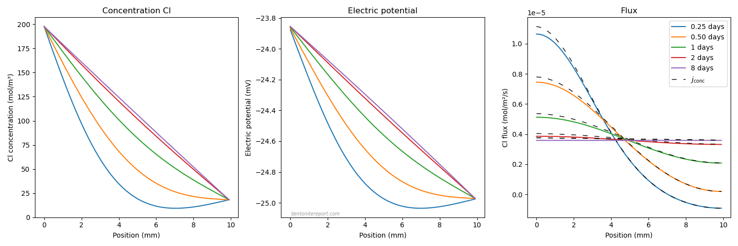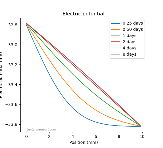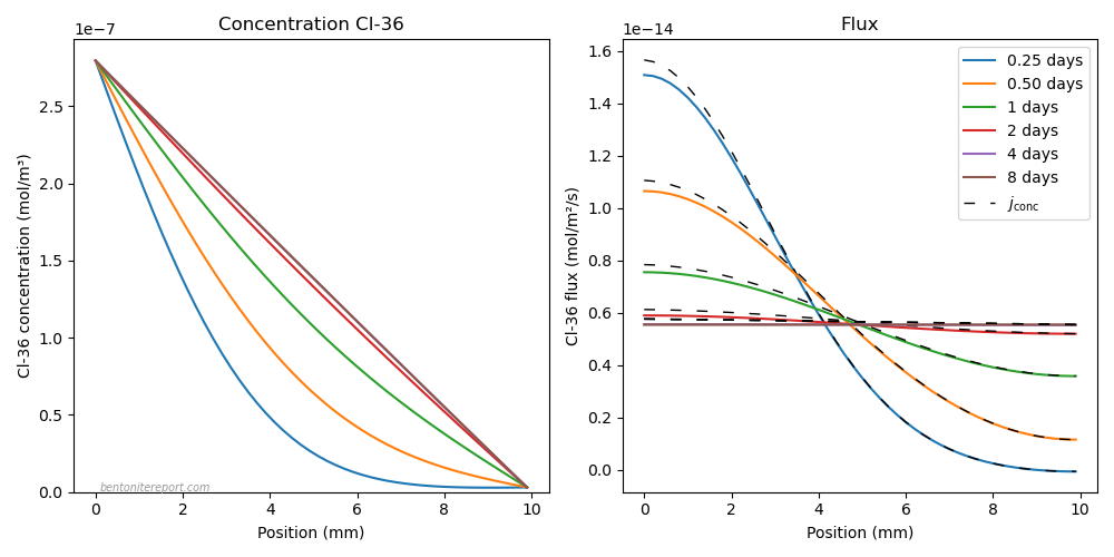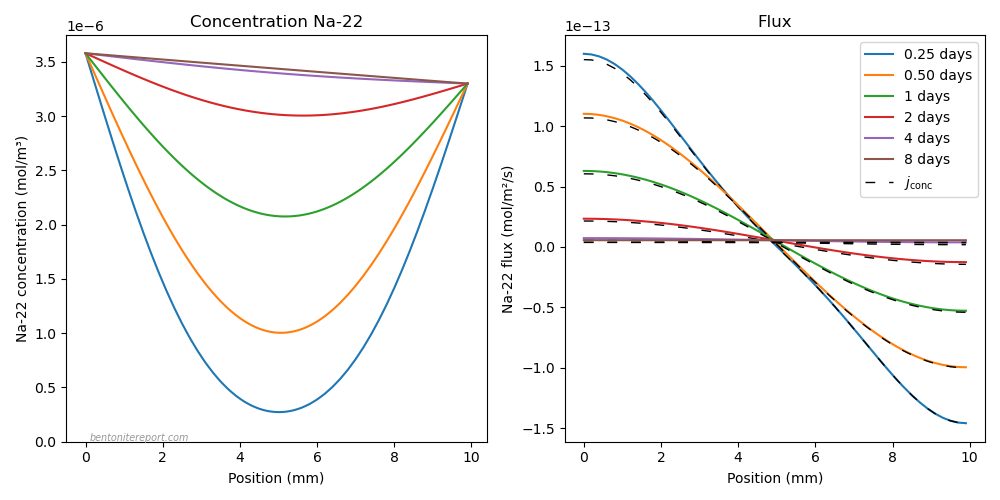
We have discussed the seeming steady-state uphill test frequently on the blog. What I find important to clarify is that the “uphill” effect is governed by the exact same mechanism that controls the behavior of cation diffusion in conventional through-diffusion tests: Donnan equilibrium.¹ This insight seems to be not at all realized in the contemporary bentonite scientific literature.

With a tool available that solves the Nernst-Planck equations in bentonite, I would here like to present a complete² modeling of the “uphill” test, with a direct comparison with the experimental results. It may also be compared with the previous evaluation, which only considered Donnan equilibrium and imposed linear concentration profiles, rather than solving the full transport equations.

Set-up

As is evident from the results of the modeling, and what we already have concluded on several occasions, the inclusion of multi-component diffusion actually makes no essential difference for the migration of the tracer in the “uphill” test. In contrast, it is crucial to include transport in the confining filters, which is to be excepted, since the test is performed with very high density montmorillonite contacted with relatively low external concentration. Likewise, the model must account for the varying concentration in the external reservoirs. Schematically the test set-up/model looks like this

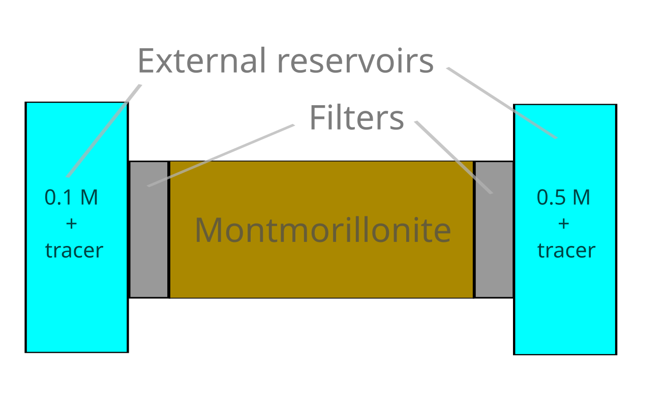
The (1D) Nernst-Planck equations are solved in the filters and the clay, and the clay is treated as a single domain with the homogeneous mixture model. Donnan equilibrium is maintained at the filter/clay interfaces.

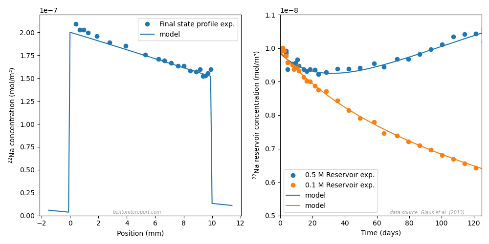
The “uphill” study (Glaus et al., 2013) presents two separate tests, where a sodium tracer diffuses in pure Na-montmorillonite samples of either 5.4 mm³ or 10 mm. Otherwise, the conditions are essentially identical. The left hand side reservoirs are kept at 0.1 M (NaClO₄), and the right hand side reservoirs at 0.5 M (NaClO₄). The nominal initial ²²Na tracer concentration is 10^-11 M in both reservoirs. The reservoir volumes are 100 ml for the test with a 10 mm sample and 250 ml for the 5.4 mm test.

Results

Here is a comparison between model and experiment for the 10 mm sample, for the final state concentration profile (after 162 days) and the evolution of the tracer concentration in the two reservoirs

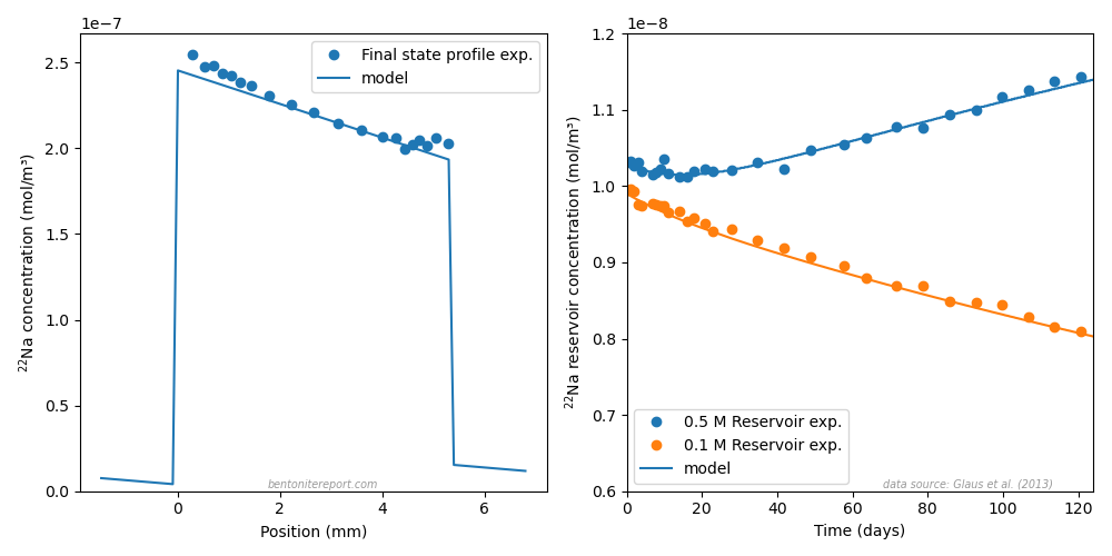
The corresponding plot for the 5.4 mm sample looks like this

The model parameters are

Sample	10 mm	5.4 mm
Porosity	0.321	0.321
\(c_\mathrm{IL}\) (CEC)	5.64 M (0.954 eq/kg)	6.21 M (1.05 eq/kg)
Cross section area	5.15 cm2	5.15 cm2
\(D_\mathrm{Na}^\mathrm{clay}\)	2.0⋅10-11 m2/s	1.9⋅10-11 m2/s
\(D_\mathrm{ClO_4}^\mathrm{clay}\)	2.67⋅10-11 m2/s	2.53⋅10-11 m2/s
Filter length	1.5 mm	1.5 mm
Filter porosity	0.321	0.321
\(D_\mathrm{Na}^\mathrm{filter}\)	6.0⋅10-11 m2/s	7.4⋅10-11 m2/s
\(D_\mathrm{ClO_4}^\mathrm{filter}\)	8.0⋅10-11 m2/s	9.9⋅10-11 m2/s
Volume reservoirs	100 ml	250 ml
\(c^\mathrm{res1}_{tr}\) (initial)	0.99⋅10-8 mol/m3	0.99⋅10-8 mol/m3
\(c^\mathrm{res2}_{tr}\) (initial)	0.985⋅10-8 mol/m3	1.03⋅10-8 mol/m3

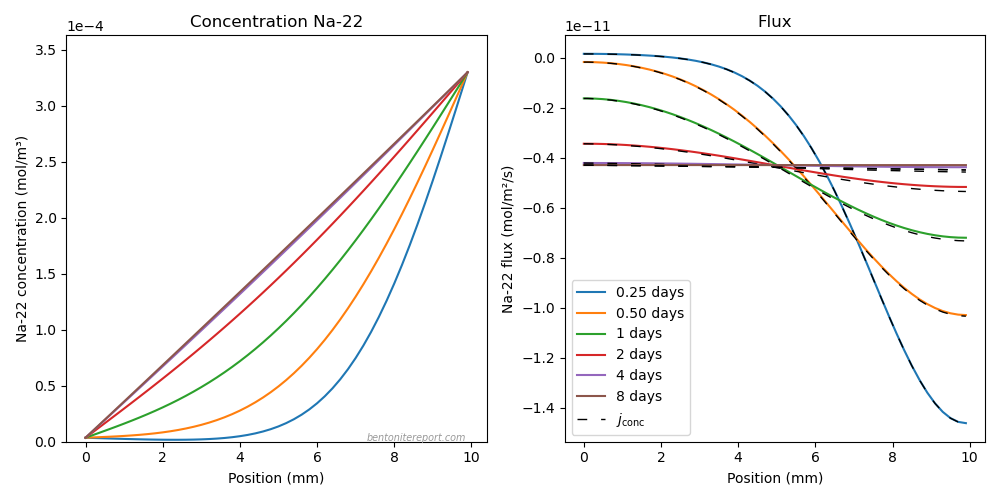
With the full model at our disposal, we can further investigate the evolution of the systems during the course of the tests. Below are plotted snapshots of tracer concentration, electric potential, and flux profiles in the 10 mm sample.

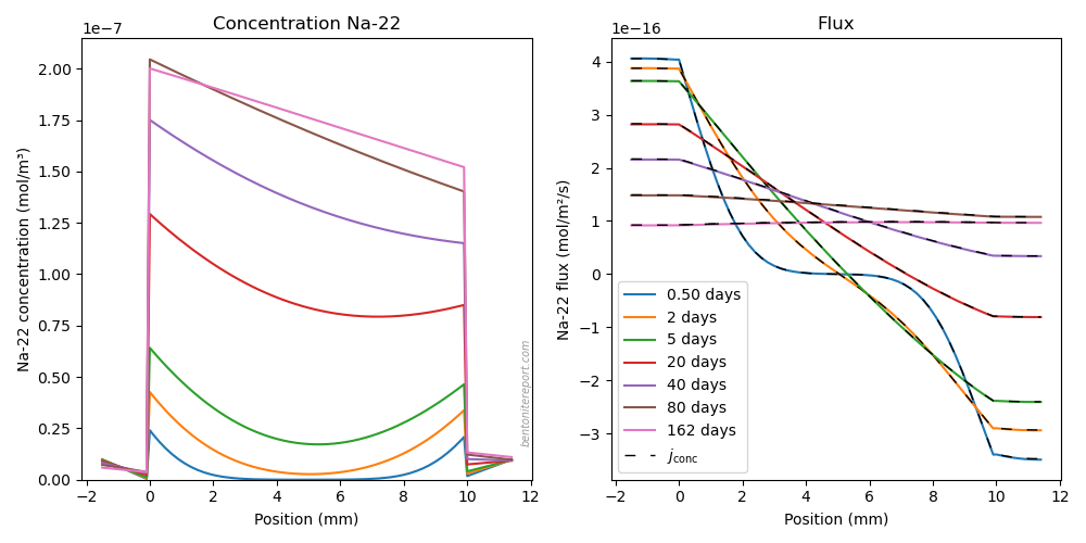
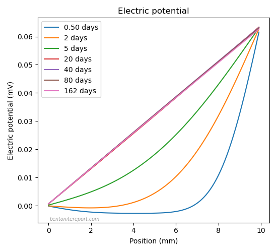
The flux snapshots show both the full flux (concentration gradient + electromigration terms) and the “Fickian” flux, i.e. the part of the flux driven by the tracer concentration gradient (dashed black lines). As in the previous assessment, we note that electromigration effects on the tracer flux is completely negligible; the flux is essentially completely “Fickian”. The diffusion potential — defined as the steady-state electric potential difference due to electromigration across the clay — is 0.06 mV.⁴ This number is even smaller than in the previous evaluation (0.09 mV), because the parameter \(c_\mathrm{IL}\) is larger here (here, \(c_\mathrm{IL}\) was used as a fitting parameter, as further discussed below).

The evolution of the Donnan potentials, and corresponding Donnan factors, at the two clay/filter interfaces look like this

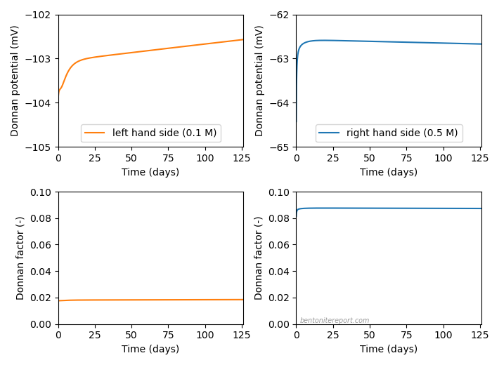
As the reservoirs have finite size, their compositions slowly change during the course of the test, and a corresponding change is seen in the Donnan potentials. As the concentration is lower in the left hand side reservoir, the change is more pronounced there. The effect on the Donnan factors (whose inverses determine the enhancement of the tracer concentrations in the clay) is nevertheless small. The contribution from Donnan equilibrium to the membrane potential — which corresponds to the difference between these Donnan potentials — evolves in the range 40.9 — 39.9 mV, in reasonable agreement with the previously evaluated (constant) contribution of 41.1 mV.⁵

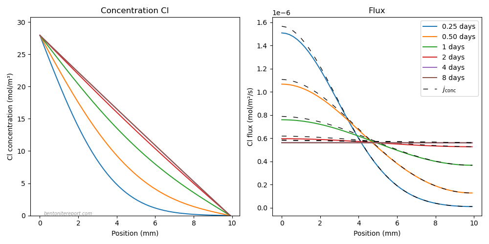
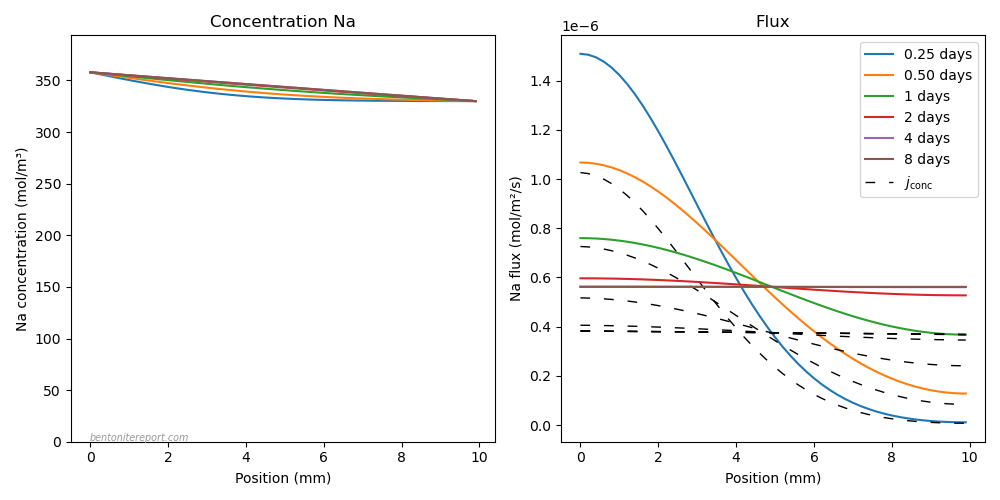
The evolution of the main salt behaves very differently as compared with the tracer

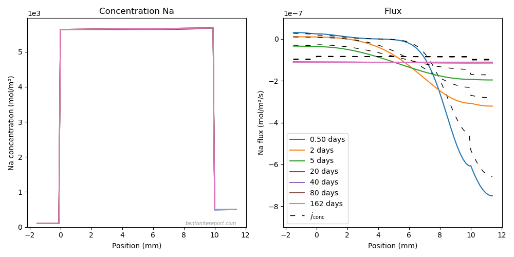
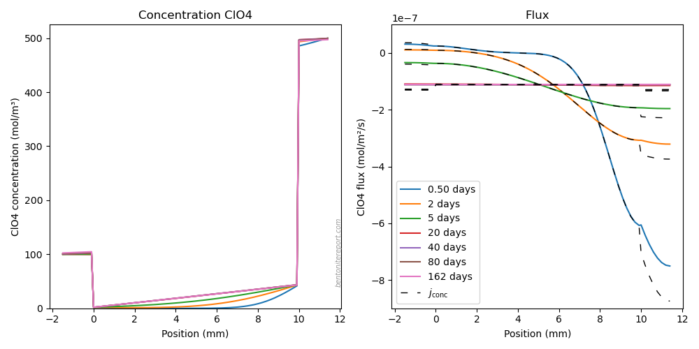
Most notably, the flux of stable NaClO₄ is directed opposite to that of the tracers (“downhill”). Note also that this flux is not limited by filter diffusivity (the concentration drop across the filters is negligible) and that this process reaches (quasi-)steady-state within 20 days. The reduced internal concentration gradient, as compared with the external concentration difference, explains why the process of equilibrating the main salt between the reservoirs is much slower in comparison to the “uphill” process. This, in turn, is of course also a consequence of Donnan equilibrium.

An electromigration effect is observed for both Na and ClO₄ in the filters (ClO₄ is beeing slowed down, while Na is boosted). In the clay (\(0 \le x \le 10\)), electromigration is mostly noticeable for sodium, because this ion has a much larger concentration there.

Fitting strategy and sensitivity analysis

We note that essentially perfect agreement can be achieved between model and experiments. But we note also that the model results depend on a quite large set of parameters. Some of these are quite easily constrained by the experiment itself, while we have used others as fitting parameters.

Regarding sample geometry, we have simply chosen the nominal density (1.9 g/cm³) and corresponding porosity (assuming a grain density of \(\rho_s\) = 2.8 g/cm³). Likewise, sample lengths and cross sectional area and reservoir volumes are fixed by what is stated in the paper.³ The filter porosity is chosen to be equal to the clay porosity, and we have chosen a filter length of 1.5 mm (as stated in Glaus et al. (2007)).

We have furthermore chosen to keep the same ratio (0.75) as for bulk solutions between sodium and perchlorate diffusivities in the montmorillonite.

The main factors that have been varied are the parameter \(c_\mathrm{IL}\) (which can be considered equivalent with varying the cation exchange capacity), the sodium diffusivity in clay (\(D_\mathrm{Na}^\mathrm{clay}\)) and filters (\(D_\mathrm{Na}^\mathrm{filter}\)), and the initial reservoir tracer concentrations (\(c_\mathrm{tr}^\mathrm{res1}\), \(c_\mathrm{tr}^\mathrm{res2}\)). For the initial tracer concentrations, it should be straightforward to accept the chosen values as evidenced by the outflux-plots. We will not comment them further.

For the sodium diffusivity in the clay, the experimental results already give a quite good hint of its value, since we can evaluate both a (quasi-)steady-state flux and a corresponding internal tracer concentration gradient. Such evaluations are naturally burdened by uncertainties, but gives a rough estimate for the sodium diffusivity of \(\sim\)2⋅10^-11 m²/s for both tests. Such a value is also expected from previous tests of sodium diffusivity in sodium montmorillonite. In particular, Glaus et al. (2007) evaluate diffusivities in nearly identical samples in the range 1.6⋅10^-11 m²/s — 2.2⋅10^-11 m²/s. Also Kozaki et al. (2005) report diffusivities of this size, albeit in a different type of sodium montmorillonite material (“Kunipia-F”).

With the clay diffusivity quite constrained there is not much choice left but to fit the model by varying the filter diffusivity (and \(c_\mathrm{IL}\)). This is the fitting strategy chosen here. In the plot below is shown the high sensitivity to the filter diffusivity in an alternative model where the filter diffusivity is increased by 20%, in the 5.4 mm sample.

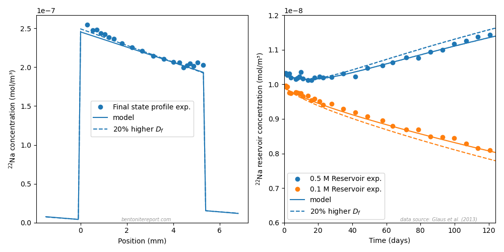
Note that the transport capacity of the filter is set by a combination of its porosity, length and diffusivity (\(\phi D/L\)). As we have no exact information on porosity and length (but keep them fixed), the filter diffusivity variation should be viewed as a variation of the filter transport capacity as a whole.

We also explore the (in)sensitivity of the multi-component aspect of the model, by investigating alternative models where the Na/ClO₄ diffusivity ratio is varied in the clay. The following plot demonstrates how insignificant the Nernst-Planck aspect is for the tracer, by comparing a model where the perchlorate diffusivity is increased to be a factor 4 larger than the sodium concentration, and a model where all diffusivities are put equal (thus eliminating electromigration completely).

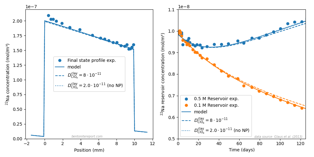
The present modeling could consequently have been done using only Fick’s laws, while giving essentially the same result (for the tracer).

The only “anomalous” parameter choice that was made in the model fittings is an unjustifiably large value of the cation exchange capacity (or \(c_\mathrm{IL}\)). The reported cation exchange capacity for the material (“montmorillonite from Milos”) is 0.8 — 0.88 eq/kg, while the fitted \(c_\mathrm{IL}\) values correspond to values approximately 10 — 30% larger. Variations of this parameter directly affects the absolute value of the internal concentration profile, but is quite insensitive to the resulting outfluxes, as seen here in a variation of the 5.4 mm model using a tabulated value for the CEC (0.85 meq/kg, \(c_\mathrm{IL}\) = 5.02 M).

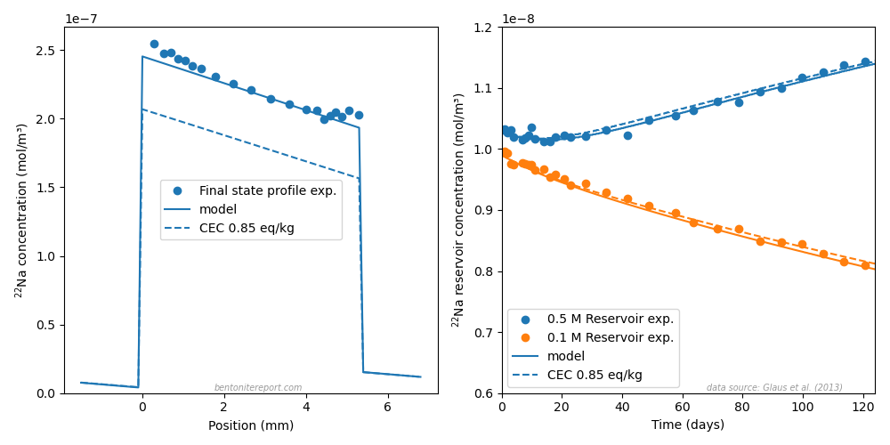
This mismatch may indicate that some effect or process is missing or not properly handled in the models. However, we should keep in mind that we have assumed the nominal density when converting the reported tracer concentration profiles (which have unit mol/kg dry clay) to pore concentrations (mol/m³). At these very high densities, \(c_\mathrm{IL}\) is hyper sensitive to the exact water-to-solid mass ratio, \(w\) (\(c_\mathrm{IL}\) depends on the inverse of \(w\)). An actual density of the samples somewhat lower than the nominal value may thereby explain the discrepancy. We may also note that the fitted \(c_\mathrm{IL}\) value varies significantly for the two tests, which also may indicate that this mismatch is a matter of experimental uncertainty, rather than being an indication of an actual effect. A further investigation of this possible anomaly would be much helped by results from additional tests.

Conclusions

• The fundamental mechanism behind the seeming uphill diffusion effect is Donnan equilibrium, just as for conventional cation through-diffusion.
• Effects of electromigration for the tracer is negligible, even though non-negligible concentration differences are maintained across the clay (and, consequently, multi-component diffusion is active).
• Donnan equilibrium also explains the negligible transport of the main electrolyte; the time scale for equilibrating the main salt across the reservoirs is much larger than the time scale of the tests.
• Filter transport limitations strongly influence the overall process.
• The only possible unexplained feature of the modeling is an indication of a too large cation exchange capacity required to perfectly fit the data (an approximate 10 — 30% increase).
• As I have whined about before, I think it is a pity that only a single study exists that explores this effect. More empirical input — e.g. for lower densities, other concentration configurations, other ion types, and membrane potentials — will greatly help process understanding.

Footnotes

[1] Someone might perhaps object to this and claim that the relevant mechanism is ion exchange. But ion exchange is nothing but a manifestation of a system that is progressing towards Donnan equilibrium. And any talk in this context about “sorption”, “sites”, surface complexation, Stern layers, immobilization, etc., is just that: talk.

[2] It’s of course dangerous to call a model “complete”. In it current state, the model still ignores e.g. pressure (but is at least in principle able to describe swelling).

[3] The nominal size of one sample is 5 mm, but it is clear from the concentration profile presented in Glaus et al. (2013) that it is slightly longer than this. In the model, we have adopted the length 5.4 mm and will here refer to it as the 5.4 mm sample.

[4] Interestingly (perhaps), the potential drop across the filters are actually comparable with that across the clay.

[5] As the Donnan potentials does not stay completely constant, we have set the reference such that \(\psi(0) = 0\) in the the plot showing the evolution of the electric potential in the clay. It would otherwise be hard to visualize, since its variation is so small.

I have started developing a tool that numerically solves the Nernst-Planck equations in bentonite on a 1D grid. It treats the bentonite within the homogeneous mixture model, accounting for the structural clay charge via the parameter \(c_\mathrm{IL}\). It also handles external solution reservoirs of finite size, and Donnan equilibrium is maintained dynamically at the interfaces between clay and external solutions. At the moment, the tool does not account for activity coefficients.

The expression for the flux of a specific species in the Nernst-Planck framework is

\begin{equation} j = j_\mathrm{conc} + j_\mathrm{E}\tag{1} \end{equation}

with the concentration concentration contribution (the “Fickan” part)

\begin{equation} j_\mathrm{conc} = -\phi\cdot D_c\cdot\nabla c^\mathrm{int}\tag{2} \end{equation}

and the electromigration contribution (driven by the induced electric field)

\begin{equation} j_\mathrm{E} = -\phi\cdot z\cdot c\cdot D_c\cdot \nabla\tilde{\psi} \tag{3} \end{equation}

Here \(D_c\), \(z\) and \(c^\mathrm{int}\) are the diffusion coefficient, charge number and concentration, respectively, for the considered species. \(\phi\) denotes porosity. For convenience, we denote the spatial derivative (\(\partial/\partial x\)) by \(\nabla\). \(\tilde{\psi}\) is the dimensionless electric potential,¹ whose gradient is

\begin{equation} \nabla\tilde{\psi} = -\frac{\sum z_i\cdot D_{c,i}\cdot \nabla c^\mathrm{int}_i} {\sum z_i^2\cdot D_{c,i}\cdot c^\mathrm{int}_i }\tag{4} \end{equation}

where the summations are over all involved charged species. Eq. 4 follows from requiring zero electric current.

The developed tool uses eqs. 1 — 4 and solves the corresponding continuity equations²

\begin{equation} \phi\cdot\frac{\partial c^\mathrm{int}_i}{\partial t} = -\nabla\cdot j_i\tag{5} \end{equation}

With this tool we can continue investigating e.g. the evolution of the electric potential in bentonite diffusion tests, as we begun in the latest blog post in the semi-permeability series.

Test case: CaCl₂ through-diffusion

As we noted previously, compacted bentonite often only show minor effects of electromigration, with diffusion potentials below 1 mV. This is because substantial counter-ion concentrations reduce the size of the electric field required to counteract effects from differences in ion mobilities (the denominator in eq. 4 is always large). To see some effect when exploring the full solution of the Nernst-Planck equation, let’s therefore focus on one of the hypothetical, “extreme” cases considered in the previous post. This test case considers diffusion of CaCl₂ through bentonite of quite low density (\(c_\mathrm{IL}\) = 1.5 M), with a 10 times lower calcium mobility relative to chloride, and has a 0.25 M CaCl₂ reservoir on the left side and a 0.05 M CaCl₂ reservoir on the right side.

In the previous consideration we did not solve the full Nernst-Planck problem (eqs. 1 — 5), but imposed a linear concentration gradient across the clay and calculated the corresponding electric potential (eq. 4) and contributions to the flux (eqs. 2 and 3). For the “extreme” CaCl₂-case, the results of this approach looked like this (relevant model parameters are summarized below the figures)

The concentration gradient contributions to the fluxes are constant throughout the clay domain (dashed lines), signifying the imposed linear concentration profile. In contrast, the total fluxes varies significantly (full lines), indicating that the system is not in steady-state. As the calcium mobility is 10 times lower than the chloride mobility, it is no surprise that the calcium flux is dominated by the electromigration contribution (dotted lines). Also the chloride flux is seen to be significantly influenced (retarded) by the electric field. The diffusion potential was evaluated to -12.1 mV, while the Donnan contribution to the membrane potential is +18.8 mV, giving an evaluated membrane potential of +6.7 mV (for a fuller discussion on these potentials, see the previous post). But note that this “membrane potential” is not completely accurately evaluated, as the linear concentration profile does not correspond to steady-state.

By solving the full Nernst-Planck framework (eqs. 1 — 5), we can investigate the size of the error in the above treatment. The full solution looks like this

This figure shows snapshots of profiles of the chloride concentration, the electric potential and the chloride flux at 0.25, 0.5, 1, 2 and 8 days; the initial condition is a chloride free calcium clay. In the flux diagram are plotted both the full flux (solid lines) and the concentration gradient contribution³ (dashed lines). Although only barely noticeable, the steady-state has a slightly non-linear concentration profile, resulting in a varying “Fickian” flux contribution (\(j_\mathrm{conc}\)). However, compared with the case with imposed linear concentration profiles, the diffusion potential changes only slightly, to -12.2 mV, giving a true steady-state membrane potential of +6.6 mV.

Below are compared the steady-state fluxes for both calcium and chloride with the fluxes evaluated from imposing linear concentration profiles.

The — now constant — total Cl flux is 3.64⋅10^-6 mol/m²/s, to be compared with a variation between 3.0⋅10^-6 mol/m²/s and 4.5⋅10^-6 mol/m²/s in the previous calculation. Likewise, the previously constant chloride concentration gradient flux of 4.88⋅10^-6 mol/m²/s now varies between approximately 6⋅10^-6 mol/m²/s and 4⋅10^-6 mol/m²/s.

We should remind ourselves that we have considered an “extreme” case, and also take a look at a more realistic/relevant model, to illustrate the often quite insignificant contribution of electromigration in bentonite. In the plot below we are solving the full Nernst-Planck framework for CaCl₂ through diffusion, as previously, but now with a denser clay (\(c_\mathrm{IL}\) = 3.0 M) and by setting the Cl/Ca diffusivity ratio equal to the corresponding value in bulk water (2.57).

We considered also this case in the previous treatment. The diffusion potential is here -1.1 mV, and the membrane potential +18.8 mV, which we also evaluated previously. Also the steady-state fluxes are essentially the same as previously evaluated: the chloride steady-state flux is 3.6⋅10^-6 mol/m²/s, while in the case with an imposed linear concentration profile, the total flux varies between 3.5⋅10^-6 mol/m²/s and 3.6⋅10^-6 mol/m²/s. All of these similarities are of course a manifestation of that the linear concentration profiles are very close to being the true steady-state profiles.

Note how similar the concentration gradient contribution is to the total flux for chloride during the entire process, in contrast to the behavior in the “extreme” case. This indicates that chloride here essentially show “Fickian” diffusion, at the rate set by its individual diffusion coefficient. It should be remembered, however, that the full transport process is still influenced by electromigration, since charge neutrality is required (the slower calcium ions are “boosted” by the electric field). But such effects are in principle no different from how salts generally diffuse in ordinary solutions.

The examples in Tournassat and Steefel (2015)

Let’s also take a new look at “example 2” and “example 3” in Tournassat and Steefel (2015), which we discussed quite thoroughly in the review of this paper.

In the original publication, these examples consider a clay component consisting of parallel bulk water and “diffuse layer” domains, and linear concentration profiles are imposed in the bulk water; a main NaCl concentration decreases from 0.1 M to 0.001 M in both examples, while different ²²Na and ³⁶Cl concentrations are maintained. In “example 2”, the tracer concentrations decrease in proportion with the main bulk electrolyte, from 10^-9 M to 10^-11 M. In “example 3” the bulk water tracer concentrations are kept at a constant value 10^-9 M.

Here we instead consider only the “diffuse layer” domain, and impose the bulk water concentrations as boundary conditions. The “diffuse layer” domain is characterized by the parameter \(c_\mathrm{IL}\) = 0.33 M (Tournassat and Steefel (2015) call this quantity \(q\)) and is assumed initially free of chloride and tracers. Solving the full Nernst-Planck equations gives the following evolution of the electric potential (this is the same for both examples)

The diffusion potential is -1.0 mV, and is comparable to the potential difference we evaluated when reviewing Tournassat and Steefel (2015). The membrane potential is +115.2 mV.

For “example 2”, the concentration and flux evolution for the tracers looks like this

In this example, the steady-state flux of both the chloride and the sodium tracer mimics the flux of the main electrolyte; the steady-state flux is the same for both species (5.6⋅10^-15 mol/m²/s) and a factor 10⁸ smaller than for the main electrolyte (5.6⋅10^-7 mol/m²/s). As the clay incorporates much more ²²Na than ³⁶Cl in the transient stage, the initial fluxes are considerably larger for ²²Na. The ³⁶Cl flux is in essence completely “Fickian”, i.e. differences between total fluxes and the concentration gradient contributions are negligible. The steady-state ²²Na flux, in contrast, has a non-negligible contribution from electromigration, in the same proportion as the stable sodium (this is not resolved in the figure above, but looks qualitatively the same as for the stable sodium, displayed below). These results are completely in line with what we earlier have concluded for the flux of these tracers.

For “example 3”, the tracer concentration and flux evolution looks like this

The evolution for ³⁶Cl is basically the same as for “example 2”. This is expected, as the right hand side boundary conditions set the clay concentration at this interface to effectively zero in both cases. The behavior of ²²Na, on the other hand, is very different as compared with “example 2”. Now a huge ²²Na concentration (relatively speaking) is established at the right hand side boundary, which results in a flux in the opposite direction with much larger magnitude (the steady-state flux is -4.3⋅10^-12 mol/m²/s). This illustrates the mechanism behind the seeming uphill diffusion effect. Note that the ²²Na flux in this case is essentially completely “Fickian” during the entire simulation.

These simulations thus confirm what we concluded in the review: all “diffuse layer” tracer fluxes in the examples in Tournassat and Steefel (2015) are essentially “Fickian”, regardless of what is stated and concluded in that publication. Likewise, the “uphill” diffusion effect does NOT rely on any significant flux contributions from electromigration.

The only significant effect of electromigration in this model is, as we have concluded previously, for the transport of the main electrolyte sodium (or the corresponding ²²Na transport in “example 2”, which mimics the main sodium flux). The concentration and flux evolution for main chloride and sodium looks like this (this is the same in both examples).

Footnotes

[1] \(\tilde{\psi}\) is normalized by the thermal voltage as \(\tilde{\psi} = \psi/V_T\), where \(V_T = RT/F\). Here we adopt \(V_T\) = 25.7 mV.

[2] The corresponding description for Fickian diffusion in the homogeneous mixture model is found here.

[3] The concentration gradient contributions to the fluxes (\(j_\mathrm{conc}\)) in the diagrams presented here are not color coded (but black), in order for them to be visible also when \(j \approx j_\mathrm{conc}\). I hope it is still reasonably easy to understand which flux profile corresponds to which time.

[4] Strictly, the main chloride and sodium fluxes differ ever so slightly in “example 3”, because there is also an ²²Na/stable Na exchange process ongoing. But this difference is not noticeable for the main ions, as the reservoir tracer concentrations are a factor 10⁶ — 10⁸ smaller.