Category Archives: Swelling pressure

Bentonite homogeneity: more evidence from cation through-diffusion

I argue that the only significant pore type in water saturated compacted bentonite is interlayers, by which I mean pores where the exchangeable cations reside (together with any other dissolved species). From this perspective it naturally follows that a homogeneous view is a suitable starting point for modeling compacted bentonite. I have presented, used, and discussed the homogeneous mixture model in many places on the blog, the main sources being

For reasons I can’t get my head around, a homogeneous view of compacted bentonite is not the mainstream in contemporary bentonite research. Instead we are stuck with “the mainstream view”, which postulates several distinctly different pore structures within the bentonite; in particular, the mainstream view uses a bulk water phase as a starting point and also distinguishes between “outer” and “inner” basal surfaces. Electric double layers are assumed to only exist on “outer” surfaces, while the function of the “inner” basal surfaces is mostly shrouded in mystery.

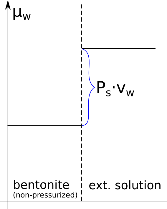
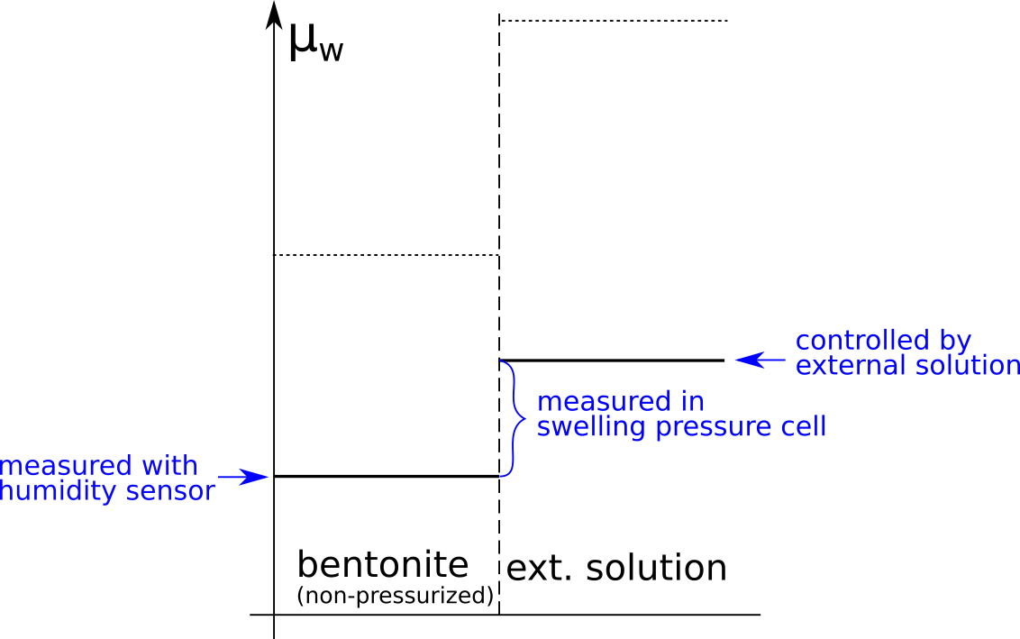
On the blog I have also presented plenty of experimental support for a homogeneous view. A main argument is that the conditions for swelling pressure — the most profound feature of bentonite in equilibrium with an external solution — are essentially fulfilled automatically in the homogeneous mixture model. The mainstream view, in contrast, requires handling of the seemingly contradictory situation of having swelling pressure while the water chemical potential is supposedly restored without pressurization. Proponents of the mainstream view often deal with this by simply ignoring swelling phenomena altogether.

I have also on the blog dissected several studies that argue for a non-homogeneous view, but that actually provide evidence for the opposite when examined more carefully. Consider in particular:

Glaus et al. (2007)

To discuss further evidence for homogeneity, we turn to one of the most profound bentonite studies published on this side of 2000: “Diffusion of \(^{22}\mathrm{Na}\) and \(^{85}\mathrm{Sr}\) in Montmorillonite: Evidence of Interlayer Diffusion Being the Dominant Pathway at High Compaction” (Glaus et al. 2007).

By systematically varying background concentration, material, and diffusing tracer, Glaus et al. (2007) clearly demonstrate, not only that the exchangeable cations are mobile, but that they dominate the flux in through-diffusion tests in highly compacted montmorillonite. While this certainly is an argument for that compacted bentonite is homogeneously structured, Glaus et al. (2007) still analyze their results from the perspective of the mainstream view, and do not — in my view — fully conclude what their results imply.

In particular they postulate the presence of an interlayer domain and a “free pore water” domain, and write for the “total” flux¹ (their eq. 3)

\begin{equation} J_\mathrm{tot} = J_\mathrm{il} + J_\mathrm{pw} \tag{1} \end{equation}

where \(J_\mathrm{il}\) is a presumed diffusive flux in the interlayer domain and \(J_\mathrm{pw}\) is the presumed diffusive flux in the “free pore water” domain.

Their subsequent analysis shows that the measured flux in montmorillonite scales as

\begin{equation} J_\mathrm{tot} \propto \frac{1}{\left ( C_\mathrm{bkg.}\right )^Z} \tag{2} \end{equation}

where \(C_\mathrm{bkg.}\) is the concentration of the background electrolyte (NaClO₄), and \(Z\) is the charge number of the diffusing tracer (\(Z = 1\) for sodium and \(Z=2\) for strontium). Moreover, by considering ion exchange equilibrium, Glaus et al. (2007) show that also \(J_\mathrm{il}\) is expected to scale according to eq. 2. As they also confirm that this scaling behavior is not observed in systems without interlayer pores (kaolinite), they could have confidently concluded that their results imply that interlayers are the only significant pore structure in montmorillonite at these densities (as the title suggests).

Unfortunately, the discussion part of the article is considerably more tentative, focusing mainly on “interpretations” of the resulting flux

The present work shows that the interpretation of cation diffusion experiments in highly compacted swelling clays in terms of the concentration gradient in the aqueous phase may result in a nonsensical dependence of the effective diffusion coefficients on the salt concentration in the external aqueous phase. An alternative interpretation using an effective diffusion coefficient in the interlayer water (\(D_\mathrm{il}\)), being independent of the external salt concentration, with a corresponding concentration gradient in the interlayer water is more consistent with the experimental observations.

and the article ends on a quite apologetic note

The proposed interpretation should in turn not be blindly applied to other experimental conditions. Diffusion of cations via the free pore water may become increasingly important in swelling clays with lower degrees of compaction or in clays in which the interlayer gel pores are not that adjacent as they are in compacted montmorillonite. In such cases, the assumption of \(J_\mathrm{tot} \cong J_\mathrm{il}\) may no longer hold, and a double-porous diffusion model would have to be applied in such cases. The present concept may also reach its limits when dealing with cations that rather sorb by surface complexation than by ion exchange. Further work is therefore planned to extend the investigations to such systems.

Given that the mainstream view to this day continues to be the default approach, one may think that this “further work” did show some convincing evidence for e.g. “diffusion of cations via the free pore water” at lower density. But what has actually been shown is that the “assumption of \(J_\mathrm{tot} \cong J_\mathrm{il}\)“ continues to be true for lower density!

Before we look at the additional results, we summarize the findings of Glaus et al. (2007).

Findings in Glaus et al. (2007)

In the following we will consider the so-called “effective diffusion coefficient”, here strictly defined as the experimental parameter

\begin{equation} D_e = -\frac{j_\mathrm{ss}\cdot L}{\Delta c^\mathrm{ext}} \tag{3} \end{equation}

where \(j_\mathrm{ss}\) denotes the steady-state flux when an external tracer concentration difference \(\Delta c^\mathrm{ext}\) is maintained across a bentonite sample of length \(L\). We have discussed through-diffusion and the role of \(D_e\) in many places on the blog, but in the present discussion we simply view \(D_e\) as a normalized version the steady-state flux.

Note that we are required to compare diffusive fluxes in different montmorillonite samples (an alternative test protocol is suggested below). \(D_e\) varies both due to varying background concentration (which is our object of study) and due to the variation of different samples. It is thus crucial to minimize the latter type of variation. This should be done (I suppose) by employing as identical preparation protocols as possible. We will get back to this complication of sorting out signal from noise as we comment the results.

Glaus et al. (2007) present their results in diagrams where the logarithm of the evaluated quantities (diffusion parameters) is plotted against background concentration. This is of course convenient, as e.g. \(D_e\) can be expected to vary by two orders of magnitude as the background concentration is varied between 0.01 M and 1.0 M. But to remind ourselves what the actual dependency looks like between the normalized steady-state flux and background concentration, I will here insist on plotting the results in lin-lin diagrams.

The results for sodium in Glaus et al. (2007) plotted in lin-lin diagrams, look like this (the data is the same in these three diagrams)

We see that the data comply with the scaling law (eq. 2) and is quite well constrained (click on pictures to enlarge). \(D_e\) is evaluated in two ways in Glaus et al. (2007): by examining at the breakthrough curve, and by examining at the internal tracer profile at test termination. These methods of evaluation give more or less identical results, with the exception of the test performed at 0.01 M background concentration. In this low concentration limit, the confining filters increasingly restrict the flux, making it difficult to extract actual clay transport parameters. We have discussed this issue (and this particular study) at length in a previous blog post.

Even with the problem of accurately measuring \(D_e\) at the lowest background concentration, the results clearly demonstrate the behavior of a homogeneous system (eq. 2): e.g., \(D_e\) undoubtedly increases by a factor of approximately 10 when the background concentration is lowered from 1.0 M to 0.1 M.

The data for strontium in Glaus et al. (2007) only covers the background concentration interval 0.5 M — 1.0 M, and is consequently less constrained, as seen here

This data also has the peculiarity that the diffusivity of samples of length 5.4 mm is almost twice as large as for samples of length 10.4 mm. This clearly demonstrates how sample preparation becomes crucial when conducting these types of tests. In the plots above, I have allowed myself to treat samples of different length separately (Glaus et al. (2007) use average values). It is clear from the data, that also strontium is compatible with the scaling law of eq. 2. In particular, it can be distinguished that sodium and strontium have different dependencies.

The take away message from these results is clear: montmorillonite at this density (1950 kg/m³) behave as a homogeneous system and show no indication of containing additional pore structures.

Glaus et al. (2013) and NTB-17-12

After the publication of Glaus et al. (2007), corresponding results for lower densities has been presented. Glaus et al. (2013) — which is mostly recognized for demonstrating the seeming “uphill” diffusion effect — also contains measured \(D_e\) of sodium as a function of background concentration in conventional through-diffusion tests, both for density 1600 kg/m³ and 1300 kg/m³. These results are also published in more detail,² together with new strontium results, in the NAGRA technical report NTB-17-12. We therefore look at these two publications together.

The additional data for sodium is here compared with the results from Glaus et al. (2007)

For some of the additional tests, both through- and out-diffusion were performed. These points are labelled “TD” and “OD”, respectively, in the diagrams. We see that even for density as low as 1300 kg/m³, the data complies with the behavior of a homogeneous system (eq. 2) and is quite well constrained; in particular, there is nothing in the data for 1300 kg/m³ that suggests that these systems behave principally different than the 1950 kg/m³ samples.

For the system at 1300 kg/m³ and background concentration 0.1 M, two different values of \(D_e\) are presented in NTB-17-12. Only the lower of these values (\(7.0\cdot 10^{-10}\) m²/s) was published in Glaus et al. (2013), but NTB-17-12 presents a continued analysis that includes filter resistance, giving the value of \(D_e\) presented in the diagram. I think this is quite interesting, as the tests made at 0.1 M used “flushed” filters in order to minimize filter resistance. Apparently, filter resistance is still influential and it is not that easy to “design away” this problem.

NTB-17-12 also presents measured values of \(D_e\) for strontium under similar conditions (1300 — 1900 kg/m³, 0.1 — 1.0 M NaClO₄ background), and are here compared with the earlier results

Although it naturally contains some scatter, we note that the additional data for ~1900 kg/m³ strengthens the earlier conclusion that also strontium scales in accordance with eq. 2. And just as for sodium, we see that the behavior does not qualitatively change, even for densities as low as 1300 kg/m³.

In the above diagrams are plotted single values for \(D_e\) for strontium at the lowest background concentration (0.1 M). It should be noted that these are burdened with large uncertainties as the transport restriction of the confining filters is severe; in NTB-17-12 are presented a whole set of simulations of the underlying flux evolution and concentration profiles with variations of the filter transport parameters. It is thus very clear that the problem of eliminating transport restrictions at the sample interfaces are not easy to completely eliminate. This is not surprising, as the theory suggests that \(D_e\) increases without limit with decreasing background concentration. Note that this behavior is strongly enhanced for divalent strontium; the measured values are many times larger than the corresponding diffusivity in bulk water (\(0.79\cdot 10^{-9}\) m²/s).

Even if the value of \(D_e\) is quite uncertain at the lowest background concentration, the mere observation that filter diffusivity strongly influence the process is, in a sense, itself a confirmation that the system still is governed by the behavior of interlayers.

The picture is quite clear from these findings: the combined results of Glaus et al. (2007), Glaus et al. (2013) and NTB-17-12 validates a homogeneous view of compacted bentonite, at essentially any relevant density!

The curious case of Bestel et al. (2018)

Bestel et al. (2018) further examine how \(D_e\) for sodium varies with background concentration. This publication shares some of the same authors with the previous studies, and presents additional measurements of \(D_e\) for sodium in essentially identical systems (similar preparation protocols, “Milos” montmorillonite, NaClO₄ background electrolyte, flushed filters). Given the substantial evidence for homogeneous behavior collected in the publications discussed above, I find the conclusions of Bestel et al. (2018) rather odd.

Bestel et al. (2018) perform subsequent measurements of the steady-state flux in the same samples at different temperatures. The dependency of \(D_e\) on background concentration, however, looks essentially the same for each temperature, and — just as Bestel et al. (2018) — we here focus mainly on the results for 25 \(^\circ\mathrm{C}\). This data looks like this³

In their analysis, Bestel et al. (2018) include the results from Glaus et al. (2007) and Glaus et al. (2013), but treat them separately. They consequently conclude implicitly that, although the earlier studies found that \(D_e\) depends on background concentration in accordance with eq. 2, the new results show a different behavior. Specifically, they conclude that \(D_e\) scale with background concentration as \(C_\mathrm{bkg}^{-0.52}\) for density 1300 kg/m³ and as \(C_\mathrm{bkg}^{-0.76}\) for density 1600 kg/m³. Bestel et al. (2018) write

The results obtained in the present work for a broad variety of bulk dry densities of Na-montmorillonite and concentrations of the background electrolyte, give clear evidence that the equilibrium distribution of cations between the clay phase and the external aqueous phase is the main parameter influencing the observed overall diffusive fluxes of cations. Whether the observed overall diffusive fluxes are described by a physical subdivision of the pore space into domains containing different species (e.g. the model proposed in Appelo and Wersin (2007) or Bourg et al. (2007)), or whether they are the result of the concentration gradients of such species in a single type of pore (e.g. the model proposed by Birgersson and Karnland (2009)), cannot be decided unambiguously from the available data — notably because of the wide similarity of the model predictions and because of some internal inconsistencies in the experimental data. Both types of models would require some adjustments in order to fully match the data. The diffusion data of \(^{22}\mathrm{Na}^+\) can equally be described by a surface diffusion model with a reduced, but non-zero mobility of sorbed cations, similar to the median value determined in Gimmi and Kosakowski (2011).

I think this is a problematic way of arguing and presenting data.

The data obviously has scatter

To begin with, why are the results from this study and the ones from Glaus et al. (2007) and Glaus et al. (2013) treated separately? When treated separately — according to Bestel et al. (2018) — these results are vaguely supposed to be incompatible: the dependence of \(D_e\) either comply with eq. 2 or it does not. I think that the appropriate thing to do is to discuss possible causes for why the new results supposedly differ from the earlier ones. As we have made clear above, all factors that determine \(D_e\) are not fully controlled in tests like these (e.g, what causes the difference in diffusivity for strontium in 5.4 mm and 10.4 mm samples, respectively, in Glaus et al. (2007)?). We have also seen that it is difficult to make accurate measurements at low enough background concentration, even with flushed filters.

Look e.g. at the specific values of \(D_e\) at background concentrations 1.0 and 0.1 M, respectively, in NTB-17-12 and Bestel et al. (2018) (unit is m²/s).

Study	1300 kg/m³ 0.1 M	1300 kg/m³ 1.0 M	1600 kg/m³ 0.1 M	1600 kg/m³ 1.0 M
NTB-17-12	\(8.6\cdot 10^{-10}\)	\(0.59\cdot 10^{-1 0}\) \(0.64\cdot 10^{-10}\)	\(3.3\cdot 10^{-10}\)	\(0.43\cdot 10^{-1 0}\) \(0.44 \cdot 10^{-10}\)
Bestel et al. (2018)⁴	\(4.5\cdot 10^{-10}\)	\(1.2\cdot 10^{-1 0}\) \(1.0\cdot 10^{-10}\)	\(3.4\cdot 10^{-1 0}\) \(3.5\cdot 10^{-10}\)	\(0.53\cdot 10^{-1 0}\) \(0.50\cdot 10^{-10}\)

Under ideal conditions, these values would not differ for the same conditions in the two studies. The scatter of these values is moreover quite random, e.g. one study do not have values that are systematically larger than in the other. In Bestel et al. (2018) we also see that the mere disturbance of a sample in form of a temperature pulse may alter the diffusivity significantly (temperature is first increased in steps from 25 \(^\circ\mathrm{C}\) to 80 \(^\circ\mathrm{C}\), then decreased in steps to 0 \(^\circ\mathrm{C}\), and finally increased again to 25 \(^\circ\mathrm{C}\)). In e.g. one sample of density 1600 kg/m³ and background concentration 0.1 M is reported \(D_e = 3.4\cdot 10^{-10}\) m²/s at 25 \(^\circ\mathrm{C}\) before the conducted temperature changes, and \(2.3\cdot 10^{-10}\) m²/s after. One should also consider that the samples are not prepared equally, as they are saturated directly with the corresponding background solution. (This is also true for the previous studies.) Could this cause differences in diffusivity?

Bestel et al. (2018) should thus either argue for why the new results are more accurate (or why the results of Glaus et al. (2007, 2013) are less accurate) or treat the data from all studies in accumulation and admit substantial experimental uncertainty. My impression is that Bestel et al. (2018) make a little of both.

The data still complies with a homogeneous view

Looking at the aggregated sodium data, a somewhat different picture emerges

Here is also included a model labelled “Full Donnan”, which takes into account the excess salt that is expected to enter the interlayers. For all other samples we have discussed, this contribution is only minor and can be neglected, and this assumption underlies eq. 2. For the sample of density 1300 kg/m³ with background concentration 5.0 M, however, the excess salt is not negligible and must be included in the analysis of the behavior of a homogeneous system (the deviation from eq. 2 is seen to become significant around 1.0 M background concentration). Bestel et al. (2018) actually present a full Donnan calculation for the excess salt, but, for unknown reasons, do not compare it directly with the experimental results (it is plotted in a separate diagram next to the data).

For 1300 kg/m³, I would claim that the “Full Donnan” model fits better to the accumulated data than the scaling law suggested in Bestel et al. (2018) (exponent \(-0.52\)). For 1600 kg/m³, the suggested scaling law (exponent \(-0.76\)) indeed fits better to the data than eq. 2, but the data is not that well constrained. To use this singular result to argue for a non-homogeneous bentonite structure basically boils down to claiming that the values measured at 0.1 M — a concentration range that is documented to be difficult to measure accurately — could not possibly be underestimated by, say, 50% (while also ignoring all other results).

If we also consider the results for strontium presented in NTB-17-12, I mean that the only reasonable conclusion that Bestel et al. (2018) can draw is that the results comply with a homogeneous bentonite structure.

Additional model components should not be motivated solely by the ability of a model to be fitted to some arbitrary data

A major motivation for measuring how \(D_e\) depends on background concentration at lower densities, according to Glaus (2007), is that “the assumption of \(J_\mathrm{tot} \cong J_\mathrm{il}\) may no longer hold”. What (I mean) has been demonstrated in the subsequent studies is that this assumption actually does hold. In particular, from the aggregated data it is not possible to claim that the behavior of \(D_e\) is qualitatively different at 1950 kg/m³ and 1300 kg/m³. Thus, there is no valid justification for introducing more complex model components. Moreover, introducing e.g. a bulk water phase causes fundamental conflicts with the description of other well-established properties of these systems, particularly swelling pressure. Adding such components merely to improve agreement with a specific dataset, while ignoring their broader implications, undermines the model’s overall coherence and validity. The data cannot “equally be described by a surface diffusion model”.

What does some alternative model actually predict?

Eq. 2 (or a full Donnan calculation) is a clean statement of the expected behavior of a homogeneous system (based on how interlayers function). If actual deviations from this behavior could be established we may conclude that a homogeneous description is not sufficient. However, any arbitrary deviation from eq. 2 does not automatically validate any specific alternative model. Validating a model requires that we can experimentally reproduce some of its non-trivial predictions. Bestel et al. (2018) don’t discuss what the exponents \(-0.52\) and \(-0.76\) are suppose to represent.

Note also that the arbitrary exponent \(-0.52\) is inferred by fitting to the data at 5.0 M background concentration. But we saw above that a full Donnan calculation within the homogeneous view actually explains the behavior in this concentration limit (Bestel et al. (2018) show this!). We have thus every reason to believe that the exponent \(-0.52\) is just spurious and do not represent some actual physical mechanisms.

We should also keep in mind that any reasonable validity of the model of Gimmi and Kosakowski (2011) has not been demonstrated, not even by the data supplied in that particular publication. I have written a separate blog post on this issue.

A suggestion for how to preferably conduct these types of tests

The discussed studies are enough to convince me that cation tracer diffusion behave in accordance with a homogeneous bentonite view at any relevant density.

It is however also clear that the full variation of \(D_e\) in these tests is caused by more factors than just background concentration and density. To eliminate as much as possible of this scatter — and thus to more accurately determine the dependence of background concentration on \(D_e\) — I suggest the following test protocol.

Measure tracer flux at several background concentrations in the same sample.

This would eliminate both the unavoidable (small) variation in density between different samples as well as several unknown factors that determine the exact value of diffusivity (these may e.g. be related to variation in material or equipment and to sample handling)
Prepare samples by saturating them all with the same low concentration solution (e.g. 0.05 M).

To me it seems reasonable that the way samples saturate may influence the resulting detailed structure and thus the diffusivity. By saturating all samples in the same manner with the same solution will minimize variations from such effects.
Keep temperature constant.

I don’t think this is a crucial factor, but we see in Bestel et al. (2018) that larger temperature pulses may significantly alter the diffusivity.
Increase background concentration in steps and record the steady-state flux at each concentration.

I think a good range may be between 0.2 M and 1.0 M. For a homogeneous system, this corresponds to a variation in \(D_e\) by a factor 5 for monovalent and 25 for divalent cations.⁵ At the same time, the problem of filter transport resistance can hopefully be kept under control.
Decrease the background concentration (perhaps in steps) back to the first concentration where steady-state flux was measured.

Measure steady-state flux again and assert that no significant change in \(D_e\) has occurred as a consequence of the disturbance introduced by the background concentration pulse.

Final thoughts

The only reasonable conclusion to draw from the studies we have looked at is that the behavior of cation tracer diffusion indicates a relatively homogeneous structure, dominated by interlayers, in any relevant bentonite system. Despite this, the contemporary scientific bentonite literature is crammed with non-homogeneous descriptions of compacted bentonite, centered around a bulk water phase (the “mainstream view”). As we have seen here, this can even be the case for studies that provide evidence for homogeneity.

What I find most frustrating is that interlayer effects often are viewed as some additional feature to be handled in specific cases. In reality, virtually all experimental findings (diffusion, swelling pressure, temperature response, Donnan effects, fluid flow, hyperfiltration, …) indicate that the behavior of compacted bentonite is fully governed by interlayers. The question is not if a presumed bulk water phase may dominate under certain conditions, but if such a phase is at all relevant. I want to emphasize this point: up until this day, no convincing evidence has ever been presented that compacted bentonite contains significant amounts of bulk water.

Even if the structure becomes more complex at lower densities, a homogeneous model centered around interlayers guarantees to cover at least some aspects of the system. On the contrary — if the goal is process understanding — most experimental evidence rules out bentonite models that assume a bulk water phase.

Footnotes

[1] We here ignore that diffusive fluxes are not additive.

[2] As far as I can see, these tests were done in duplicates for Na diffusion with background concentrations 0.5 M and 1.0 M, and the the numbers reported in Glaus et al. (2013) are averages.

[3] Bestel et al. (2018) use a normalization scheme in their analysis that involves corresponding measured water diffusivities and parameters from “Archie’s law” (note, it is the quotation marks version of the law). I think this handling makes the presented results less transparent, and here we use the actual reported values of \(D_e\).

[4] These are only values from the first phase at 25 \(^\circ\mathrm{C}\).

[5] I assume that measurements are being made in pure Na-montmorillonite.

Post-publication review: Tournassat and Steefel (2015), part II

Leave a reply

This is the second part of the review of “Ionic Transport in Nano-Porous Clays with Consideration of Electrostatic Effects” (Tournassat and Steefel, 2015) (referred to as TS15 in the following). For background and context please check the first part. That part covered the introduction and the section “Classical Fickan Diffusion Theory”. The next section is titled “Clay mineral surfaces and related properties”, and is further partitioned into two subsections. Here we exclusively deal with the first one of these subsections: “Electrostatic properties, high surface area, and anion exclusion”. It only covers three and a half journal pages, but since the article here goes completely off the rails, there is much to comment on.

“Electrostatic properties, high surface area, and anion exclusion”

As stated in the first part, I find it remarkable that the authors use general terms such as “clay minerals” when the actual subject matter is specifically systems with a significant cation exchange capacity, and montmorillonite in particular. I will continue to refer to these systems as “bentonite” in the following, disregarding the constant references to “clay minerals” in TS15.

Stacks

After having established that montmorillonite and illite have structural negative charge, it begins:

Clay mineral particles are made of layer stacks and the space between two adjacent layers is named the interlayer space (Fig. 5).

This is the first mention of clay “particles” in the article, and they are introduced as if this is a most well-established concept in bentonite science (incredibly, it is also the first occurrence of the term “interlayer”). We will refer to “clay mineral particle” constructs as “stacks” in the following. I have written a detailed post on why stacks make little sense, where I demonstrate their geometrical impossibility and show that most references given to support the concept are studies on suspensions that often imply that montmorillonite do not form stacks. Sure enough, this is also the case in TS15

The number of layers per montmorillonite particle depends on the water chemical potential and on the nature and external concentration of the layer charge compensating cation (Banin and Lahav 1968; Shainberg and Otoh 1968; Schramm and Kwak 1982a; Saiyouri et al. 2000)

Banin and Lahav (1968), Shainberg and Otoh (1968), and Schramm and Kwak (1982) all report studies on montmorillonite suspensions. The abstract of Shainberg and Otoh (1968) even states “The breakdown of the tactoids occurred when the equivalent fraction of Na increased from 0.2 to 0.5. Montmorillonite clay saturated with 50% calcium (and less) exists as single platelets.”, and the abstract of Schramm and Kwak (1982) states “Upon exchange of Ca-counterions for Li-, Na-, or K-counterions, a sharp initial decrease in tactoid size was observed over approximately the first 30% of cation exchange.”. These are just different ways of saying that sodium dominated montmorillonite is sol forming.

I want to stress the absurdity of the description given in TS15. A pure fantasy is stated about how compacted bentonite is structured. As “support” for the claim are given references to studies on “dilute suspensions”. It should be clear that the way TOT-layers interact in such suspensions essentially says nothing about how they are organized at high density. But even if we pretend that these results are applicable, the given references say that most of the relevant systems (montmorillonite with about 30% sodium or more) do not form stacks.

Disregarding the references, note also how bizarre the above statement is that the number of layers in a “particle” depends on “the water chemical potential and on the nature and external concentration of the layer charge compensating cation”: stacks are supposed to be fundamental structural units, yet the number of layers in a stack is supposed to depend on the entire water chemistry?! (It makes sense, of course, for stacks in actual suspensions.) Also, for montmorillonite an actual number of layers is nowhere stated in TS15.

TS15 further complicate things by lumping together montmorillonite and illite. In contrast to Na-montmorillonite, illite has by definition a mechanism for keeping adjacent TOT-layers together: its layer charge density is higher and compensated by potassium, which doesn’t hydrate that well, leading to collapsed interlayers. As far as I understand, one characterizing feature of illite is that the collapsed interlayers are manifested as a “10-angstrom peak” in X-ray diffraction measurements.

To treat montmorillonite and illite on equal footing (in a laid-back single sentence) again shows how nonsensical this description is. Stacking in montmorillonite suspensions occurs as a consequence of an increased ion-ion correlation effect when the fraction of e.g. calcium becomes large (> 70-80%). This process requires the ions to be diffusive and is distinctly different from the interlayer collapse in illite.

I actually have a hard time understanding what exactly is meant by the term “illite” here. In clay science it is clear that what is referred to by this name are systems that may have a quite considerable cation exchange capacity.¹ Reasonably, such systems contain other types of cations besides potassium² (as they are exchangeable), and must contain compartments where such ions can diffuse (as they are exchangeable). To increase the complexity, there are also “illite-smectite interstratified clay minerals”, which typically are in “smectite-to-illite” transitional states. For these, it seems reasonable to assume that the remaining smectite layers provide both diffusable interlayer pores and the cation exchange capacity. I don’t know if such “smectite layers” provides the cation exchange capacity in general in systems that researchers call illite. Neither do I understand how researchers can accept and use this, in my view, vague definition of “illite”. Anyway, it is the task of TS15 to sort out what they mean by the term. This is not done, and instead we get the following sentence

Illite particles typically consist of 5 to 20 stacked TOT layers (Sayed Hassan et al. 2006).

This study (Sayed Hassan et al., 2006) concerns one particular material (illite from “the Le Puy ore body”) that has been heavily processed as part of the study.³ I mean that such a specific study cannot be used as a single reference for the general nature of “illite particles”. Moreover, the stated stack size (5 — 20 layers) is nowhere stated in Sayed Hassan et al. (2006)!⁴

In their laid-back sentence, TS15 also implicitly define “interlayer space” as being internal to stacks. I criticized this way of redefining already established terms in the stack blog post, and TS15 serves as a good illustration of the problem: are we not supposed to be able to use the term “interlayer” without accepting the fantasy concept of stacks? To be clear, “interlayer spaces” in the context of montmorillonite simply means, and must continue to mean, spaces between adjacent TOT basal surfaces. It drives me half mad that the “stack-internal” definition is so common in contemporary bentonite scientific literature that this point seems almost impossible to communicate.

The provided illustration (“Fig 5”) explicitly shows how TS15 differ between “interlayers” that are assumed internal, and “outer basal surfaces” that are assumed external to the stack.

This illustration misrepresents the actual result of assembling a set of TOT-layers, just like any other “stack” picture found in the literature. The figure shows five identical TOT-layers that can be estimated to be smaller than 20 nm in lateral extension (while the text “conveniently” states that they should be 50 — 200 nm). Compared with “realistic” stacks, formed by randomly drawing TOT-layer sizes from an actual distribution, the depicted stack in TS15 looks like this⁵ (see here for details)

Besides the fact that “realistic” stack units cannot be used to form the structure of compacted bentonite, it should also be clear from this picture that “outer basal surfaces” and “interlayers” (in the sense of being internal to the stack) are not well defined. Note further that in actual compacted systems (above 1.2 g/cm³, say) such “realistic” stacks would be pushed together, something like this

In this picture, why should e.g. the interface between the green and the red stack be defined as an interface between two “outer surfaces” rather than an interlayer? Also, is this interface supposed to change nature and become an “interlayer”, as the water chemical potential or the external ion content changes? Like all other proponents of stack descriptions that I have encountered, TS15 do not in any way explain how “interlayers” and “outer surfaces” are supposed to function fundamentally differently. Similarly, they do not describe how the number of layers in a stack depends on water chemistry, nor do they provide a mechanism for why (sodium dominated) montmorillonite stacks of are supposed to keep together.

I want to emphasize that I do not favor any construction with “realistic” stacks, but only use them to illustrate the absurd consequences of taking a stack description seriously, and to demonstrate that all such descriptions in the bentonite literature are essentially pure fantasies, including the one given in TS15. I’m also quite baffled as to why TS15 (and others) provide such completely nonsensical descriptions, and how these can end up in review articles. I believe a hint is given in this formulation

[T]he number of stacked TOT layers in montmorillonite particles dictates the distribution of water in two distinct types of porosity: the interlayer porosity […] and the inter-particle porosity.

The only way I can make sense of this whole description is as an embarrassing attempt to motivate the introduction of models with several “distinct types of porosity”: the outcome is simply a macroscopic multi-porosity model (which will also be evident in later sections).

I’ve written a detailed blog post on why multi-porosity models cannot be taken seriously. There I point out that basically all authors promoting multi-porosity for some reason attempt to dress it up in terms of microscopic concepts, while the models obviously are macroscopic. Moreover, no one has ever suggested a mechanism for how equilibrium is supposed to be maintained between the different types of “porosities”.

Anion exclusion

After hallucinating about the structure of compacted bentonite, TS15 change gear and begin an “explanation” of anion exclusion. Let’s go through the description in detail.

The negative charge of the clay layers is responsible for the presence of a negative electrostatic potential field at the clay mineral basal surface–water interface.

I cannot really make sense of the term “negative electrostatic potential field”, although I think I understand what the authors are trying to say here. What is true is that the electrostatic potential near a montmorillonite basal surface is lowered compared to a point farther away. But whether or not the value of the potential is negative is irrelevant, as we are free to choose the reference level. If the zero level is chosen at a point very far from the surface, which often is done, it is true that the potential is negative at the surface. But the key principle is that the potential decreases towards the surface.⁶ A varying electrostatic potential signifies an electric field, which in this case is directed towards the surface (\(E = -d\phi/dx\)).

Furthermore, the electric field is not present merely because of the presence of negative charge, but because this charge is constrained to be positioned in the atomic structure of the clay. Remember that the structural clay charge is compensated by counter-ions, and that the system as a whole is charge neutral. The reason for the presence of an electric field near the surface is due to charge separation. And the reason for the potential decreasing (i.e. the electric field pointing towards the surface) is because it is the negative charge that is unable to be completely freely distributed.⁷

The concentrations of ions in the vicinity of basal planar surfaces of clay minerals depend on the distance from the surface considered. In a region known as the electrical double layer (EDL), concentrations of cations increase with proximity to the surface, while concentrations of anions decrease.

Having established that the electrostatic potential varies in the vicinity of the surface, it follows trivially that the ion concentrations also vary. I also find it peculiar to label the regions where the concentrations varies as the EDL. An electric double layer is a structure that includes both the surface charge and the counter-ions (hence the word “double”). What is described here should preferably be called a diffuse layer. Note, moreover, that the way an electric double layer here is introduced implies that TS15 consider a single interface, i.e. some variant of the Gouy-Chapman model (this becomes clear below). But this model is not applicable to compacted bentonite.

At infinite distance from the surface, the solution is neutral and is commonly described as bulk or free solution (or water).

Here I think it becomes obvious that the authors try to motivate the presence of bulk water within the clay structure. As described in the blog post on “Anion accessible porosity”, it is only reasonable to assume that diffuse layers merge with a bulk solution in systems that are very sparse — i.e. in suspensions.⁸ This is how e.g. Schofield (1947) utilized the Gouy-Chapman model to estimate surface area. But how is the solution next to a basal surface in compacted bentonite supposed to merge with a bulk solution? Even if we use the authors’ own fantasy stack constructs, the typical structure of compacted bentonite must be envisioned something like this (I have color coded different stacks to be able to understand where they begin and end).

The regions where basal surfaces of different stacks face each other (labelled A) are way too small in order to merge with a bulk solution (and, as asked earlier, how are these regions even different from “interlayers”?). Furthermore, regions adjacent to external edge-surfaces of these imaginary stack units (B, C) are not at all considered by applying a Gouy-Chapman model. The only way to make “sense” out of the present description is to imagine larger voids in the clay structure, something like this

But even if such voids would exist (in equilibrated water-saturated bentonite under reasonable conditions, they do not) they would only constitute an exotic exception to the typical pore structure. By focusing on this type of possible “anion” exclusion, TS15 completely miss the point.

This spatial distribution of anions and cations gives rise to the anion exclusion process that is observed in diffusion experiments.

Now I’m lost. I don’t understand how ion distributions are supposed to cause a process. I think the authors here allude to Schofield’s approach to estimating surface area in montmorillonite suspensions. As discussed in detail in the blog post on anion-accessible porosity, if the suspension is so dilute that we can consider each clay layer independently, and if we equilibrate it with an external solution, we can measure its salt content, and use the Gouy-Chapman model to e.g. estimate surface area from the amount of excluded salt (as compared with the external solution).

But, as also discussed in the blog post on salt exclusion, the “Schofield type” of exclusion is not what we expect to be dominating in a dense system. Rather, in denser systems (and in Donnan systems generally — no surfaces need to be involved), salt exclusion occurs mainly because of charge separation at interfaces with the external solution. I find it revealing that TS15 so far in the article has not at all mentioned such interfaces.

Moreover, in the above sentence TS15 causally states that the anion exclusion process is “observed in diffusion experiments”, without further clarification. Given that the previous section treated diffusion, a reader would expect to have been introduced to the anion exclusion process and how it is observed in diffusion experiments. But this subsection is the first time in TS15 where the term “anion exclusion” is used! In the section on diffusion, “anion accessible porosity” was briefly mentioned, and I suppose a reader is here presumed to connect the dots. But the presence of an exclusion process certainly does not imply an “anion accessible porosity”! Furthermore, anion exclusion is not necessarily observed in diffusion experiments. A more correct statement is that we observe effects of salt exclusion in experiments where a bentonite sample is contacted with an external solution via a semi-permeable component (which typically is a filter that keeps the clay in place). The effect is most conveniently studied in equilibrium rather than diffusion tests, and salt exclusion is not present in e.g. closed-cell diffusion tests. Note that exclusion effects are always related to an external solution.

As the ionic strength increases, the EDL thickness decreases, with the result that the anion accessible porosity increases as well.

Here it is fully clear that TS15 conflate “anion accessible porosity” and “anion exclusion”. If we consider the “Schofield type” of salt exclusion, it is true that the so-called “exclusion volume” changes with the ionic strength. However, an exclusion volume is not a physical space, but an effective, equivalent quantity. It is derived from the Gouy-Chapman model, which always has anions present everywhere.

Even more importantly, the “Schofield type” of exclusion is not really of interest in dense systems (nor is the Gouy-Chapman model valid in such systems). As discussed above, one must instead consider salt exclusion stemming from charge separation at interfaces with the external solution. For this case it does not even make sense to define an exclusion volume.

I can only interpret this entire paragraph as another fruitless attempt to motivate a multi-porous modeling approach. In this subsection we have so far been told that “two distinct types of porosity” can be defined (they cannot), and we have vaguely been hinted that “bulk or free solution” also is relevant for modelling compacted bentonite. And with the last quoted sentence it is relatively clear that TS15 try to establish that the relative sizes of various “porosities” are controlled by a simple parameter (ionic strength).

The final paragraph of this subsection contain several statements that makes my jaw drop.

An equivalent anion accessible porosity can be estimated from the integration of the anion concentration profile (Fig. 6) from the surface to the bulk water (Sposito 2004)

Here the authors suddenly use the phrase “equivalent”! They are thus obviously aware of that “anion accessible porosity” is a spurious concept?! ?!?! I really don’t know what to say. Their own graph (“Fig. 6”) even show that the Gouy-Chapman model has anions (salt) everywhere! Note that this statement also implies that “the bulk water” is assumed to exist within the clay.

In compacted clay material, the pore sizes may be small as compared to the EDL size. In that case, it is necessary to take into account the EDLs overlap between two neighbouring surfaces.

I think this is a very revealing passage. The conditions of compacted bentonite are treated as an exception: pore sizes “may” be smaller than the EDL, and “in that case” it is necessary to account for overlapping diffuse layers. But for compacted bentonite, this is the only relevant situation to consider! Without “overlapping” diffuse layers there is no swelling and no sealing properties. An entire page has been devoted to discussing a model only relevant for suspensions (Gouy-Chapman), while “compacted clay material” here is commented in two sentences…

Clay mineral particles are, however, often segregated into aggregates delimiting inter-aggregate spaces whose size is usually larger than inter-particle spaces inside the aggregates.

All of a sudden — in the middle of a paragraph — we are introduced to a new structural component! “Aggregates” have not been mentioned earlier in the article and is here introduced without any references. It is my strong opinion that this way of writing is not appropriate for a scientific publication, especially not for a review article. I’m not sure what type of system the authors have in mind here, but “aggregates” are typically not present in actual water saturated bentonite. I have commented more on this in the blog post on stacks.

Conclusion

At the end of the previous section (on diffusion), we were promised that this section should qualitatively link “fundamental properties of the clay minerals” to the diffusional behavior of compacted bentonite. Instead, we are given a fictional description of the structure (conflated with structures of other “clay minerals”), along with a confused explanation of anion exclusion that is irrelevant for such systems. Not a single word is said about the equilibrium that must be considered, namely that at interfaces between bentonite and external solutions. Rather, the idea of “overlapping” diffuse layers — which is the ultimate cause for bentonite swelling — is treated as an exception and only commented on in passing (and nothing is said about how to handle such systems). Although nothing is fully spelled out, I can only interpret this entire part as a (failed) attempt to motivate a multi-porous approach to modeling bentonite. And multi-porosity models cannot be taken seriously.

I admit that scrutinizing studies and pointing out flaws can be fun. However, considering that the descriptions in TS15 are the rule rather than the exception in contemporary bentonite research, I mostly feel weary and resigned. I don’t mean that every clay researcher must agree with me that a homogeneous model is the only reasonable starting point for describing compacted bentonite, and I could only wish that this blog was more influential. But I feel almost dizzy thinking about how this research sector is so hermetically sealed that one can spend entire careers in it without ever having to worry about understanding the nature of swelling and swelling pressure.

Update (250901): Part III of this review is found here.

Footnotes

[1] The Wikipedia article on illite, for example, states that the cation exchange capacity is typically 0.2 — 0.3 eq/kg. Is a significant cation exchange capacity required for classifying something as illite?

[2] E.g. (Poinssot et al., 1999), that TS15 reference as a source on illite, work with sodium exchanged “illite du Puy”, i.e. “Na-illite”.

[3] The material was dispersed by diluting it in alkaline solution and sonicating it. It was thereafter dropped as a suspension on a glass slide and dried.

[4] We may note that the number 5 — 20 TOT-layers in a stack actually showed up when we investigated how this concept is (mis)used in descriptions of bentonite. There it turned out to be a complete misunderstanding of the behavior of suspensions of Ca-montmorillonite.

[5] I am not capable to produce anything reasonable in 3D, but I think a 2D representation still conveys the message.

[6] Perhaps this criticism can be regarded as nitpicking. I have a nagging feeling, though, that electrostatics is quite poorly understood in certain parts of the bentonite research field. Take the phrase “negative electrostatic potential field”, for example. Although it can be understood at face value (a scalar field with negative values), it also appears to mix together stuff related to charges (“negative”), electric fields (“field”), and potentials. It certainly is important to separate these concepts. There are many examples in the clay literature when this is not done. E.g. Madsen and Müller-Vonmoos (1989) mean that two “potential fields” can repel each other (and also misunderstand swelling)

A high negative potential exists directly at the surface of the clay layer. […] When two such negative potential fields overlap, they repel each other, and cause the observed swelling in clay.

Horseman et al. (1996) claim that a potential repels charges:

[…] the net negative electrical potential between closely spaced clay particles repel anions attempting to migrate through the narrow aqueous films of a compact clay […]

And Shackleford and Moore (2013) mean that “overlapping” potentials repel charges

In this case, when the clay is compressed […] to the extent that the electrostatic (diffuse double) layers surrounding the particles overlap, the overlapping negative potentials repel invading anions such that the pore becomes excluded to the anion.

[7] An isolated layer of negative charge of course also has an electric field directed towards it, but this is not the relevant system to consider here. (Such a system will actually have an electric field strength that is independent of the distance to the surface, as long as the layer can be regarded as infinitely extended.)

[8] See also this comment, and this quotation.

Sorption, part V: A case against Stern layers

Leave a reply

It should go without saying that modelers and model developers must justify every feature, mechanism, or component that they use. Failing to do so strongly increases the risk of being fooled by overparameterization rather than gaining insight. The bentonite scientific literature is nonetheless full of incorrect or unjustified model assumptions, several of which have been discussed previously on the blog. Examples include assuming the presence of bulk water, assuming “stack” structures, and assuming that diffusive fluxes from separate domains are additive. Here we discuss yet another unjustified common model component: Stern layers on montmorillonite basal surfaces.

In the bentonite literature, a Stern layer essentially means a layer of “specifically” sorbed ions on the basal surface, as e.g. illustrated here, in a a figure very similar to what is found in Leroy et al. (2006). Illustrations like this are ubiquitous in the literature.

If montmorillonite basal surfaces function roughly as uniform planes of charge we expect the counter-ions to form a diffuse layer, as e.g. described by the Gouy-Chapman model. By introducing a Stern layer, however, many bentonite researchers mean that exchangeable cations in general also interact with basal surfaces by forming immobile surface complexes. Such interactions necessarily involve mechanisms more “chemical” than the pure electrostatic interaction with uniform planes of charge, and the typical description postulates localized “sorption sites”, as illustrated above.

This blog post treats three different main arguments against Stern layers, presented in different sections

Lack of a coherent description of the surface chemistry
Deviations from the Gouy-Chapman model have other causes
Experimental evidence of counter-ion mobility

I want to make clear that this criticism concerns one particular type of surface: the montmorillonite basal surface. Stern layer models are found in many research fields dealing with solid interfaces, and although they have been criticized more generally, here we have no intention of doing so. Likewise, the process of surface complexation is certainly important generally — even in bentonite, e.g. on edge surfaces of montmorillonite particles.¹

To better be able to criticize the use of Stern layers on basal surfaces in bentonite modeling, we begin by discussing the origin of Stern’s model.

Origins of the Stern Layer model

The Stern layer concepts were introduced by Otto Stern² as an extension of the Gouy-Chapman model. Stern’s main concern was metallic electrodes in electrochemical applications. In such systems, the surface (electrode) potential is externally controlled, and can typically be on the order of 1 volt. It is easily seen that the Gouy-Chapman model predicts nonsense for such surface potentials. For e.g. a 1:1 system, the counter-ion concentration at the surface is enhanced by a factor of the order of \(10^{17}\)(!), as seen directly from the Boltzmann distribution \(c^\mathrm{surf} = c^\mathrm{ext}\cdot e^{e\psi^0/kT}\), where \(\psi^0\) is the surface potential, \(e\) is the elementary charge, \(kT\) the thermal energy, and \(c^\mathrm{ext}\) is the concentration far away from the surface. The main problem is that the Gouy-Chapman model does not account for the finite size of ions, and therefore can accumulate an arbitrary amount of charge at the surface. To remedy this flaw, Stern suggested to divide the interface region into a “compact” layer and a “diffuse” part, with the division located an ionic radius from the electrode surface (sometimes referred to as the outer Helmholtz plane).

In the simplest version of Stern’s model the compact layer is free of charges but act as a plate capacitor with a prescribed capacitance (per unit area) \(K_0\). In the original paper Stern shows that, with electrode potential \(\psi^0 = 1\) V and external 1:1 solution concentration \(c^\mathrm{ext} = 1\) M, such a capacitive layer reduces the potential where the diffuse layer begins to \(\psi^1 = 0.08\) V; lowering the external concentration to \(c^\mathrm{ext} = 0.01\) M gives \(\psi^1 = 0.18\) V. For these calculations, Stern uses a value of \(K_0 = 0.29\;\mathrm{F/m^2}\), adopted from measurements on mercury electrodes. This version of the Stern model is essentially a way to take into account that ions cannot get arbitrarily close to the surface.

Stern also presented more elaborate versions of the model that include adsorption in the compact layer (as a Langmuir adsorption model). It is such mechanisms that is universally referred to as a Stern layer in the bentonite scientific literature. Clearly, such versions are substantially more conceptually complex; rather than to just account for a finite ion size at the first molecular layer, we must now also consider additional chemical interactions that typically are different for different types of ions. We also need to have an idea about the adsorption capacity.

Lack of a coherent description of “specific sorption” on montmorillonite basal surfaces

When using Stern layers for describing montmorillonite basal surfaces, a first thing to note is that the surface potential is not independently controlled for these systems. In contrast to metallic electrodes, montmorillonite is characterized by a fixed surface charge and the problem of accumulating unrealistically large amounts of ions at the interface is significantly mitigated. As pointed by e.g. Norrish and Bolt already in the 1950s, even if we put all counter-ions within the first nanometer adjacent to the surface, the corresponding ion concentration is not larger than approximately 3 M. Here is a illustration of the montmorillonite basal surface on the nm scale, with a representative number of monovalent counter-ions (top layer oxygen atoms are red and the counter-ions blue).³

Clearly, there is room to accommodate all ions without running into the problems that was initially addressed by Stern’s model. Of course, solely accounting for the finite size of the ions — as is done in the simplest version of Stern’s model — is always well justified and will in principle improve the description. In particular, a pure diffuse layer model overestimates the capacitance of the surface. As shown in the table below, the introduction of an empty Stern layer “fixes” this problem.

\(c^\mathrm{ext}\) (M)	\(\psi^1\) (V)	\(c^1\) (M)	\(\psi^0\) (V)	\(K_\mathrm{Stern}\) (\(\mathrm{F}/\mathrm{m ^2}\))	\(K_\mathrm{DL}\) (\(\mathrm{F}/\mathrm{m ^2}\))
0.001	0.206	3.57	0.590	0.188	0.538
0.01	0.148	3.59	0.532	0.209	0.748
0.1	0.092	3.77	0.475	0.234	1.212
1	0.042	5.39	0.426	0.260	2.612

Here \(c^\mathrm{ext}\) is the concentration of the 1:1 salt far away from the surface, \(\psi^1\) and \(c^1\) denote the electrostatic potential and the counter-ion concentration, respectively, at the point where the diffuse layer begins (i.e. at the interface to the compact layer), and \(\psi^0\) is the electrostatic potential at the surface. \(K_\mathrm{Stern}\) denotes the corresponding capacitance as calculated from the Stern model, with the choice \(K_0 = 0.29 \;\mathrm{F/m^2}\). \(K_\mathrm{DL}\) is instead the capacitance as calculated from a pure diffuse layer model (in which case the surface potential has the value of \(\psi^1\)). In the calculations are assumed a montmorillonite surface charge of 0.111 \(\mathrm{C}/\mathrm{m ^2}\).

But to simply account for the finite size of the ions by means of an empty compact layer is not how the term Stern layer is used in the bentonite scientific literature. As mentioned, most bentonite researchers mean that parts of the rather sparse collection of ions on the surface interacts chemically (“specific sorption”, “chemisorption”). The question of whether Stern layers on montmorillonite basal surfaces are well motivated thus reduces to what arguments there are for more elaborate chemical mechanisms being active on these surfaces. And descriptions of specific sorption on basal surfaces are really all over the place.

Deshpande and Marshall (1959, 1961) claim that counter-ions are partitioned between (i) chemisorbed ions, which do not contribute to conductivity or activity, (ii) physisorbed ions in a Stern layer, which do not contribute to activity or D.C. conductivity, and (iii) diffuse layer ions, which contribute fully to activity and conductivity. If I interpret their numbers correctly, they state that about 75% — 80% of the counter-ions in pure K-montmorillonite are immobilized. Note that these authors mean that ions in the Stern layer are “physically” adsorbed, while the surface also has “chemically” adsorbed species. Thus, they use the term Stern layer for certain types of physisorption, while stating that ions also bond covalently to the surface.

Shainberg and Kemper (1966, 1967), on the other hand, model ions as either mobile in a diffuse layer or immobile in a Stern layer. They argue that covalently bound ions are “extremely unlikely”, and mean that ions in the Stern layer form “ion pairs” with the surface, as suggested earlier by Heald et al. (1964). They use this idea as a starting point for analyzing differences in exchange selectivity for different monovalent cations in montmorillonite. They claim that “about 20 to 50% of sodium are specifically adsorbed”.

Note that Shainberg and Kemper, just like Deshpande and Marshall, assume Stern layer ions to be “physically” bonded to the surface (i.e. non-covalently), while having a completely different opinion on the presence of chemisorbed ions. Shainberg and Kemper (1966) provide a picture showing the conceptual difference between an ion in the Stern layer (“unhydrated”) and ions in the diffuse layer (“hydrated”) that looks very similar to this

In this context it may be worth to also mention the work of Low and co-workers. Low argued consistently that swelling pressure is not primarily related to the exchangeable ions — something that I strongly disagree with and that I commented briefly on in a previous blog post.⁴ Directly related to this view, these authors claim that the exchangeable ions for the most part do not dissociate from the surfaces, and in later papers they refer to such ions as being part of a Stern layer.

To me, all the above descriptions seem like little more than speculation. None of these authors discuss how or why e.g. sodium ions (!) are supposed to from ion pairs with a charge center buried far inside the montmorillonite layer, nor how or why they bond covalently with the basal surface. Nevertheless, both Low as well as Shainberg and Kemper seem to have influenced the writings of Sposito, who, in turn, has had quite a huge impact on contemporary descriptions of bentonite. In e.g. Sposito (1992), which specifically discusses montmorillonite (“smectite”), he writes

Despite the long history of continual investigation of the surface and colloid chemistry of smectites (van Olphen, 1977; Sposito, 1984), the structure of the electrical double layer at smectite surfaces and its influence on the rheological properties of smectite suspensions remain topics of lively controversy. One of the most contentious issues is the partitioning of adsorbed monovalent cations among the three possible surface species on the basal planes of smectite particles, such as montmorillonite (see, e.g., Low, 1981, 1987). […] [A] monovalent cation can be adsorbed on the basal planes by three different mechanisms: inner-sphere surface complexes, in which the cation desolvates and is captured by a ditrigonal cavity; outer-sphere surface complexes, in which the cation remains solvated but still is captured by a ditrigonal cavity and immobilized; and the diffuse-ion swarm, in which the cation is attracted to the basal plane, but remains fully dissociated from the smectite surface (Sposito, 1989a, Chap. 7).

The view conveyed here is that exchangeable ions do not interact with montmorillonite basal surfaces as if these, to a first approximation, are planes of uniform charge. Such interaction is only supposed to govern an outer diffuse layer (called a “diffuse-ion swarm” for unclear reasons), and ions are also supposed to interact with the surface by no less than two other “mechanisms”, related to the “ditrigonal cavities”.

Note that while Sposito acknowledges an ongoing “lively controversy” regarding how to describe montmorillonite basal surfaces, he specifies that this debate is limited to how to distribute the exchangeable ions among “three possible surface species.” But, as we will explore below, there is certainly no consensus within colloid chemistry that exchangeable ions are involved in complexation chemistry on the basal surfaces! (I therefore find this way of formulating the “controversy” quite dishonest, to be honest.) For reasons I can’t get my head around, descriptions of “inner-” and “outer-sphere complexes” on montmorillonite basal surfaces are anyway ubiquitous in modern bentonite literature. Let’s therefore take a closer look at how these are introduced.

“Inner-” and “outer-sphere” surface complexes

A description that hardly enlightens me is given in Sposito (1989)⁵

[The inner- and outer-sphere complexes] constitute the Stern layer on an adsorbent. […] The diffuse-ion swarm and the outer-sphere surface complex mechanisms of adsorption involve almost exclusively electrostatic bonding, whereas inner-sphere complex mechanisms are likely to involve ionic as well as covalent bonding. Because covalent bonding depends significantly on the particular electron configurations of both the surface group and the complexed ion, it is appropriate to consider inner-sphere surface complexation as the molecular basis of the term specific adsorption. Correspondingly, diffuse-ion screening and outer-sphere surface complexation are the molecular basis for the term nonspecific adsorption. Nonspecific refers to the weak dependence on the detailed electron configurations of the surface functional group and adsorbed ion that is to be expected for the interactions of solvated species.

Here, Sposito means that exchangeable ions bond covalently with the montmorillonite basal surface,⁶ in agreement with Deshpende and Marschall, and in disagreement with Shainberg and Kemper (we have one “extremely unlikely” and one “likely” for covalent bonding…). In contrast to Deshpende and Marschall, however, Sposito means that these “inner-sphere” complexes are part of the Stern layer. To confuse matters even more, Shainberg and Kemper assume their “unhydrated” construct (which corresponds structurally to an “inner-sphere” complex, see above figure) as being part of the Stern layer, but not part of any covalent bonding. Moreover, Shainberg and Kemper assume their “hydrated” construct (corresponding structurally to an “outer-sphere” complex, see above figure) to be part of the diffuse layer, while Sposito wants his “outer-sphere” complexes to be immobile and part of the Stern layer…

Given the above description (and others) it is hard to understand what the difference is supposed to be between an “outer-sphere” complex and an ion in the “diffuse-ion swarm”, other than that the former is simply claimed to be immobilized; both ions are said to interact with “exclusively electrostatic bonding”,⁷ both are classified as “nonspecific adsorption”, and both are fully hydrated. In my head, this is simply a recipe for achieving an overparameterized model description.

Sposito’s description also makes implicit statements about the montmorillonite basal surface: it contains “surface functional groups” whose specific electron configuration significantly influence covalent bonding, while being insensitive for the formation of “outer-sphere” complexes and the “diffuse ion-swarm”. In Sposito (1984) he suggests that the “functional groups” are groups of oxygen atoms on the surface of the montmorillonite particle (“ditrigonal cavities”) that qualifies as Lewis bases. The presence of atomic substitutions in the octahedral layer is supposed to enhance this Lewis base character

If isomorphic substitution of \(\mathrm{Al}^{3+}\) by \(\mathrm{Fe}^{2+}\) or \(\mathrm{Mg}^{2+}\) occurs in the octahedral sheet, the resulting excess negative charge can distribute itself principally over the 10 surface oxygen atoms of the four silica tetrahedra that are associated through their apexes with a single octahedron in the layer. This distribution of negative charge enhances the Lewis base character of the ditrigonal cavity and makes it possible to form complexes with cations as well as with dipolar molecules.

Note how completely different this whole description is compared to the original Gouy-Chapman conceptual view. Here is implied that montmorillonite basal planes⁸ cannot be described as a passive layer of charge, but that it is a fully reactive system, including covalent bonding mechanisms.

Frankly, I dismiss the above description of the montmorillonite surface as a Lewis base as pure speculation. I will gladly admit that I am a physicist rather than a chemist, and perhaps I am missing something obvious, but I really don’t see any argumentation behind this description. I am also under the impression that montmorillonite basal planes are relatively chemically stable — that is why they form in the first place, and that is also one reason for why we are interested in using bentonite for e.g. long-term geological waste storage. Furthermore, a meta-argument for dismissing this description is that in later publications we find statements like this, in Sposito (2004):

The \(\mathrm{Na}^+\) that are counterions for the negative structural charge developed as a result of isomorphic substitutions within the clay mineral layer tend to adsorb as solvated species on the basal plane (a plane of hexagonal rings of oxygen ions known as a siloxane surface) near deficits of negative charge originating in the octahedral sheet from substitution of a bivalent cation for \(\mathrm{Al}^{3+}\). This mode of adsorption occurs as a result of the strong solvating characteristics of Na and the physical impediment to direct contact between Na and the site of negative charge posed by the layer structure itself. The way in which this negative charge is distributed on the siloxane surface is not well known, but if the charge tends to be delocalized there, that would also lend itself to outer-sphere surface complexation.

So, 20 years after the surface chemistry of montmorillonite was described as if it was completely understood (Sposito, 1984), the way the negative charge distributes is now described instead as “not well known”… Furthermore, in contrast to earlier statements, the formation of an “outer-sphere complex” is here associated mainly with the hydration properties of sodium. But if the idea of a “surface functional group” is discarded — or at least downplayed — why should a hydrated ion near the surface be described as a surface complex at all?

We note that Sposito (2004) still seem to imply that the “outer-sphere surface complex” is localized and immobile (“adsorbed near deficits of negative charge”) But the evidence is vast that sodium, and several other ions, are quite mobile even in monohydrates (see below).

Deviations from the Gouy-Chapman model do not imply surface complexation

Authors that promote Stern layers on montmorillonite basal surfaces usually rely on the Gouy-Chapman model for describing the diffuse layer part. Lyklema, writing generally on colloid science, explicitly “defends” such an approach

In the following our discussion will be based on the rather pragmatic, though somewhat artificial, subdivision of the solution side of the double layer into two parts: an inner part, or Stern layer where all complications regarding finite ion size, specific adsorption, discrete charges, surface heterogeneity, etc., reside and an outer, Gouy or diffuse layer, that is by definition ideal, i.e. it obeys Poisson-Boltzmann statistics. This model is due to Stern following older ideas of Helmholtz and has over the decades since its inception rendered excellent services, especially in dealing with experimental systems.

Dzombak and Hudson (1995) express a similar attitude

Bolt and co-workers […] investigated in detail the application of the Gouy–Chapman diffuse-layer theory to ion-exchange processes. Their work demonstrated that consideration of electrostatic sorption alone is not sufficient to explain ion-exchange data and that chemisorption (or “specific” sorption) needs to be included in ion-exchange models.

It is not logically consistent to conclude that deviations from the Gouy-Chapman model implies that specific sorption “needs to be included”.⁹ On the contrary, introducing specific sorption to compensate for a certain model rather than for surface chemical reasons may, in my mind, be a recipe for an overparameterized disaster. I don’t get reassured by statements like this, also from Dzombak and Hudson (1995)

Surface complexation models can be extended to include diffuse-layer sorption. This approach permits their application in modeling the sorption of ions (such as monovalent electrolyte ions) that exhibit weak specific sorption. The generality of such an extended surface complexation approach together with the mathematical power of modern chemical speciation models offers the potential for accurate physicochemical modeling of ion exchange

Reasonably, a complex system may require complex models, but it is certainly dangerous in a modeling context to rely too heavily on “mathematical power” (I guess “numerical power” is the preferred phrase).¹⁰

Note that very different attitudes towards the Stern layer concept is found in the colloid science literature, where e.g. Evans and Wennerström (1999) describe it as an “intellectual cul de sac”.¹¹

One way of dealing with these difficulties is to say that the solution layer closest to a charged surface has properties so different from the bulk that it should be treated as a separate entity. This device was introduced in the 1930s by the German electrochemist Stern and the surface layer is commonly referred to as the Stern layer, whose properties are specified by a number of empirical parameters. It is the opinion of the authors of this book that the Stern layer concept is an intellectual cul de sac for the description of electrostatics in colloidal systems. One reason for this point of view is that from modern spectroscopic measurements we know molecular properties are not dramatically changed for a liquid close to a charged surface.

I find it quite perplexing that so many authors in the bentonite scientific community attribute any deviation from the Gouy-Chapman model solely to surface-related mechanisms. The Gouy-Chapman model treats both ions (point particles) and water (a dielectric continuum) in a very simplified manner, and it is clear that “specific ion” effects are ubiquitous, also in systems that lack surfaces. Addressing differences in e.g. selectivity coefficients without considering ion polarizability and hydration, while postulating the existence of localized sorption “sites”, can, to my mind, only lead to incorrect descriptions.

The Poisson-Boltzmann equation is a mean field approximation

Note also that the Poisson-Boltzmann equation — which underlies the Gouy-Chapman model — is only approximate. It is derived by assuming that the electrostatic potential experienced by any ion is the average potential from all other ions (and surfaces). More accurately, the ion distribution around a given ion deviates from the average, as a direct consequence of the presence of the central ion.

Including these ion-ion correlation effects makes the mathematical description considerably more complex. But with the advent of sufficiently powerful computers and algorithms, the electric double layer has been solved basically “exactly”. The “exact” solution may differ strongly from the Poisson-Boltzmann solution, with increasing concentrations towards the surfaces (and consequently a lowering of interlayer midpoint concentrations), and an explicit attractive electrostatic force between the two halves of an interlayer. Using Monte Carlo simulations, Guldbrand et al. (1984) demonstrated that with divalent counter-ions these effects are so large that the system becomes net attractive at a certain interlayer distance, in qualitative disagreement with the Poisson-Boltzmann solution. This effect, which has been thoroughly studied since the 80s, and which we have discussed in several posts on this blog, is the prevailing explanation e.g. for the limited swelling of Ca-montmorillonite.

The lesson here is that observed deviations from predictions of the Poisson-Boltzmann equation not automatically can be taken as evidence for additional active system components, and certainly not as evidence for specific sorption. Note that limited swelling in divalent montmorillonite is explained by the ions being diffusive, not that they are sorbed and immobilized. I cannot overstate the importance of this insight.

It boggles my mind that the entire research area on ion-ion correlations in colloidal systems seems to have made no significant impact on parts of the bentonite scientific community; I seldom find references to works on ion-ion correlation, and when I do it’s quite confused. E.g. Sposito (1992) means that the formation of “quasicrystals”¹² is due to “outer-sphere” complexes

The best known example of a montmorillonite quasicrystal is that comprising stacks of four to seven layers. \(\mathrm{Ca}^{2+}\) ions, solvated by six water molecules (outer-sphere surface complex), serve as molecular “cross-links” to help bind the clay layers together through electrostatic forces.

Sure, the ion-ion correlation effect that prevents Ca-montmorillonite from exfoliating is of electrostatic origin, but it is not related to “cross-links” or surface complexes. Sposito furthermore continues by claiming that “even […] Na-montmorillonite” forms “quasicrystals”. Such claim cannot be supported by ion-ion correlation — on the contrary, ion-ion correlation explains why Ca-montmorillonite forms “quasicrystals”, while Na-montmorillonite does not. It is thus relatively clear that Sposito do not refer to ion-ion correlation in the above statement. At the same time, later in the same publication he cites Kjellander et al. (1988) on going beyond the mean-field treatment of the Poisson-Boltzmann equation, and even claims that the Gouy-Chapman model is “completely inaccurate” for systems containing divalent ions. I can only conclude that this is a quite confused description.

Finite-size effects of water molecules

With focus on the first molecular layers at a solid interface, it is clear that finite-size effects of water molecules — which are not treated in the Gouy-Chapman model — reasonably influences the resulting ion distribution. This influence is manifested both as a steric effect — there can only be a discrete number of water molecules between the ion and the surface — and as an effect of how strongly a certain ion is hydrated.

Water molecules are treated explicitly e.g. in molecular dynamics (MD) simulations of montmorillonite/water interfaces, and here are results from simulating a three water-layer interlayer of Na-montmorillonite, from Hedström and Karnland (2012)¹³

Sodium is seen to accumulate “between” the water layers; in the above illustration we have also included schematic illustrations of the molecular configurations, as conceived by Shainberg and Kemper (1966) (shown earlier). As stated earlier, Shainberg and Kemper (1966) refer to these as “hydrated” and “unhydrated”, but they are clearly the same type of configurations that e.g. Sposito (1992) and Dzombak and Hudson (1995) call “outer-” and “inner-sphere” complexes.

While the above mentioned authors mean that these “complexes” involve specific interactions between ions and surface, the MD simulation suggests that such structures are mainly a consequence of the finite-size of the molecules and ions. In particular, the MD results do not support the idea that these structures depend critically on a specific, non-electrostatic, ion–surface interaction. Indeed, the simulations explicitly treat also the atoms of the montmorillonite layer, which could make it difficult to judge whether the appearance of “complexes” mainly is related to water–ion or ion–surface interactions. But note that Hedström and Karnland (2012) simulate two different systems: one where the montmorillonite charge is put on specific atoms in the octahedral sheet (Mg for Al substitutions), and one where it is distributed on all Al atoms (as a fraction of the elementary charge). Both systems have essentially an identical atomic configuration in the interlayer, which strongly suggest that no critical ion–surface interaction is involved in forming “outer-” and “inner-sphere complexes” (i.e. they really are not surface complexes). I am not aware of any published simulation where the basal surface is represented as a uniform sheet of charge while water molecules are treated explicitly, but I am convinced that “outer-” and “inner-sphere complexes” would appear also in such a simulation.

Regarding MD simulations of montmorillonite interlayers, you can also simply observe them to convince yourself that the counter-ions are not in any reasonable sense immobilized. These types of simulations are routinely used to calculate (quite significant) interlayer diffusion coefficients, for crying out loud!

Experimental evidence of counter-ion mobility

A final argument for why Stern layers on montmorillonite basal surfaces are unjustified is the vast amount of empirical evidence of counter-ion mobility. We have discussed several diffusion studies in earlier blog posts that show that many ions (Na, Cl, K, Sr, I, Cs, Ca,…) have a significant mobility even in very dense systems, dominated by bi- or monohydrated interlayers. In the previous post, we brought up the following result

This figure shows the resulting concentration profiles in two diffusion experiments where sodium and chloride tracers, respectively, have diffused from an initial planar source for the same amount of time (23.7 h), in samples of pure Na-montmorillonite of dry density 1.8 \(\mathrm{g/cm^3}\), equilibrated with deionized water. This result was used previously to dismiss the ludicrous idea that these two ions are supposed to migrate in separate parts of the pore volume, exposed to completely different mechanisms. In the same vein, this result can be used to dismiss the idea of a Stern layer on basal surfaces.

Sodium, which is universally acknowledged to reside in the interlayers, is here demonstrated to diffuse just fine in bi- and monohydrated interlayers. As chloride, which also resides in the interlayers (despite all talk of “anion-accessible porosity”), behave essentially identical, it is quite far-fetched to assume any significant surface complexation mechanism. And anyone who argues for that these tracers actually do not diffuse in the interlayers should be reminded of the seeming “uphill” diffusion experiment,¹⁴ which is performed at even higher density, and where the “uphill” diffusion direction once and for all proves that the transport occurs in interlayers.

Strangely, many authors nowadays seem to promote both Stern layers and interlayer mobility in bentonite. Various simulation codes has been modified for this possibility, and there are several examples of researchers pointing out a possibility of “Stern layer diffusion”. I think these authors should carefully examine their chain of assumptions: Surface complexation in a Stern layer (i.e. sorption) is initially suggested to explain e.g. why breakthrough times in cation through-diffusion tests are relatively long as compared with the steady-state flux (i.e. why “\(D_e\)” can be considerably larger than”\(D_a\)”). With evidence for that the “sorbed” ions actually dominate the mass transfer, the sorption mechanism is not reconsidered, but yet another mechanism is suggested: Stern layer mobility… Reasonably, such an approach is not adequate for developing models; researchers employing it should critically consider the intended purpose of a Stern layer component.

Counter-ion mobility is also related to swelling pressure. Bentonite swelling pressure is difficult to describe generally, and I have written a whole series of blog posts on the subject, but it is clear that measured swelling pressures in e.g. moderately dense Na- and Li-montmorillonites is quite well described by the Poisson-Boltzmann equation. As this set of conditions (not too dense clay, simple monovalent ions) are exactly those for which we expect the Poisson-Boltzmann equation to be adequate, this is a strong indication that all counter-ions contribute to the pressure.¹⁵ Also, the limited swelling in e.g. Ca-montmorillonite, as previously discussed, is explained by ion-ion correlation effects where all ions are included in the diffuse layer.

Finally, we can take a look at salt exclusion from compacted bentonite. The magnitude of salt exclusion is directly related to the amount of mobile counter-ions. Thus, if most of the counter-ions were immobilized in a Stern layer, bentonite should show small exclusion effects. In contrast, the empirical results for e.g. chloride exclusion in sodium dominated bentonite indicate, again, that all counter-ions are part of a diffuse layer.

This diagram shows the relative amount of chloride in the bentonite as a function of \(c^\mathrm{ext}/c_\mathrm{IL}\), where \(c^\mathrm{ext}\) is the external salt concentration and \(c_\mathrm{IL}\) is the amount exchangeable cations, expressed as a monovalent interlayer concentration. The experimental data is from Van Loon et al. (2007), which we reevaluated and examined in detail in a previous blog post. The lines are the result from applying the “ideal” Donnan formula with various amounts of the counter-ions assumed diffusive. For details on Donnan theory, see this blog post.

Although the experimental data show considerable scatter, there is nothing in this plot that suggests that a fraction of the counter-ions are immobilized. And the quality of this data is certainly good enough to directly dismiss models that assume that the major part of ions are immobilized in a Stern layer.

Footnotes

[1] I find it quite frustrating that many descriptions in the literature only refer abstractly to “mineral surfaces” rather than specifically addressing montmorillonite. At the same time it is often clear from the context that statements regarding “mineral surfaces” should be understood as applicable to montmorillonite basal surfaces. I would much appreciate if researchers promoting Stern layers on basal surfaces would provide descriptions for specific systems, e.g. pure Na-Ca-montmorillonite.

[2] Otto Stern is a fascinating character in the history of science, most famous for the Stern-Gerlasch experiment, that helped pave the way for quantum mechanics. I highly recommend this lecture by the late Sandip Pakvasa. An example of its contents:

A note on Stern’s style of working: He always had a cigar in one hand, and he left actual work with hands to others, as he did not trust his own manual dexterity! […] He described the beneficial effects of a large wooden hammer that he kept in his lab and used it to threaten the apparatus if it did not behave! (apparently it worked!)

[3] Note that di-valent counter-ions would be even more sparsely distributed than this.

[4] It may be worth discussing my objections against the work of Low and co-workers in more detail in a future blog post.

[5] This is a general discussion on sorption on mineral surfaces, and is cited from the second edition of the book (2008). There is also a “Thired” edition.

[6] This particular description is general (for “adsorbents”), but since Sposito, as well as a large part of the contemporary bentonite scientific community, claim that “inner-sphere” complexes are present on montmorillonite basal surfaces, we can conclude that they mean that covalent bonding occur on such surfaces.

[7] Sure, the full quotation is “almost exclusively electrostatic bonding”, but what is a reader supposed to do with that? Such vague and sloppy scientific writing annoys me.

[8] Again, the discussion is on general “mineral surfaces”, but from other writings it is clear that this is supposed to apply to the montmorillonite basal surface.

[9] I furthermore don’t believe that “Bolt and co-workers” concluded that specific sorption “needs” to be included, but that this rather is an interpretation made by Dzombak and Hudson themselves. Bolt considered and downplayed the Stern Layer already in the mid 50s, and although he indeed has expressed positive attitudes (seriously, these guys just write too much!), he continued to downplay its significance in e.g. Bolt (1979), writing “In conclusion it appears justified to assume that for homoionic clays saturated with common ions, if hydrated, the Stern layer will be an “empty” Stern layer according to the terminology of Grahame (1947).”

[10] Note also that the perspective in this quotation is that specific sorption models can be complemented with diffuse layer features — i.e. the existence of sorption “sites” is assumed a priori. But Dzombak and Hudson (1995) never really discuss the nature of such “sites” on montmorillonite basal surfaces, but rely on Sposito’s speculations about “inner-” and “outer-surface” complexes.

[11] Note that Stern’s original paper actually is from 1924. I also suspect that Stern would object to being labeled an “electrochemist”.

[12] The terminology here is quite messy, and other authors may use other terms such as “tactoids”, see this post for a further discussion.

[13] This study was thoroughly discussed in a blog post on MD simulations and anion exclusion.

[14] Anyone making this argument should also provide a plausible suggestion for where a significant non-interlayer pore structure is located at these extreme densities.

[15] The pressure in these types of calculations can be related to the interlayer midpoint concentration. But this does not mean that not all counter-ions are involved in the process.

Are interlayer cations not attracted to the surfaces?!

Leave a reply

Electrostatics can be quite subtle. The following comment on the interlayer ion distribution, in Kjellander et al. (1988), was an eye-opener for me

The ion concentration profile is determined by the net force acting on each ion. The electrostatic potential from the uniform surface charges is constant between the two walls, which means that the forces due to these charges cancel each other completely. Thus, the large counter-ion concentration in the electric double layer near the walls is solely a consequence of the repulsive interactions between the ions.

Interlayer cations are not attracted to the surfaces, but are pushed towards them due to repulsion between the ions themselves! My intuition has been that interlayer counter-ions distribute due to attraction with the surfaces, but the perspective given in the above quotation certainly makes a lot of sense. Here I use the word “perspective” because I don’t fully agree with the statement that the ion distribution is solely a consequence of repulsion. To discuss the issue further, let’s flesh out the reasoning in Kjellander et al. (1988) and draw some pictures.

Here we discuss an idealized model of an interlayer as a dielectric continuum sandwiched between two parallel infinite planes of uniform surface charge density.¹ The system is thus symmetric around the axis normal to the surfaces (the model is one-dimensional).

From electrostatics we know that the electric field originating from a plane of uniform surface charge has the same size at any distance from the plane (we discussed this fact in the blog post on electrostatics and swelling pressure). We may draw such electric fields like this

From this result follows that the electric field vanishes between two equally negatively charged surfaces. The electrostatic field configuration for an “empty” interlayer can thus be illustrated like this

This means that the two interlayer surfaces don’t “care” about the counter-ions, in the sense that this part of the electrostatic energy (ion – surfaces) is independent of the counter-ion distribution.

To consider the fate of the counter-ions we continue to explore the axial symmetry. The counter-ion distribution varies only in the direction normal to the surfaces, and we can treat it as a sequence of thin parallel planes of uniform charge. Since the size of the electric field from such planes is independent of distance, the force on a positive test charge (= the electric field) at any position in the interlayer depends only on the difference in total amount of charge on each side of this position, as illustrated here

This, in turn, implies both that the electric field is zero at the mid position, and that the electric field elsewhere is directed towards the closest surface (since symmetry requires equal amount of charge in the two halves of the interlayer²). The counter-ions indeed repel each other towards the surfaces! The charge density must therefore increase towards the surfaces, and we understand that the equilibrium electric field qualitatively must look like this³

However, as far as I see, the “indifference” of the surfaces to the counter-ions is a matter of perspective. Consider e.g. making the interlayer distance very large. In this limit, the system is more naturally conceptualized as two single surfaces. It is then awkward to describe the ion distribution at one surface as caused by repulsion from other ions arbitrarily far away, rather than as caused by attraction to the surface. But for the case most relevant for compacted bentonite — i.e. interlayers, or what is often described as “overlapping” electric double layers — the natural perspective is that counter-ions distribute as a consequence of repulsion among themselves.

This perspective also implies that anions (co-ions) distribute within the interlayer as a consequence of attraction to counter-ions rather than repulsion from the surfaces! (The above figure applies, with all arrows reversed.) This insight should not be confused with the fact that repulsion between anions and surfaces is not really the mechanism behind “anion exclusion”. Rather, the implication here is that anion-surface repulsion can be viewed as not even existing within an interlayer.

A couple of corrections

With this (to me) new perspective in mind, I’d like to correct a few formulations in the blog post on electrostatics and swelling. In that post, I write

[R]ather than contributing to repulsion, electrostatic interactions actually reduce the pressure. This is clearly seen from e.g. the Poisson-Boltzmann solution for two charged surfaces, where the resulting osmotic pressure corresponds to an ideal solution with a concentration corresponding to the value at the midpoint (cf. the quotation from Kjellander et al. (1988) above). But the midpoint concentration — and hence the osmotic pressure — is lowered as compared with the average, because of electrostatic attraction between layers and counter-ions.

But the final sentence should rather be formulated as

But the midpoint concentration — and hence the osmotic pressure — is lowered as compared with the average, because of electrostatic repulsion between the counter-ions.

In the original post, I also write

This plot demonstrates the attractive aspect of electrostatic interactions in these systems. While the NaCl pressure is only slightly reduced, Na-montmorillonite shows strong non-ideal behavior. In the “low” concentration regime (< 2 mol/kgw) we understand the pressure reduction as an effect of counter-ions electrostatically attracted to the clay surfaces.

The last part is better formulated as

In the “low” concentration regime (< 2 mol/kgw) we understand the pressure reduction as an effect of electrostatic repulsion among the counter-ions.

I think the implication here is quite wild: In a sense, electrostatic repulsion reduces swelling pressure!

Footnotes

[1] The treatment in Kjellander et al. (1988) is more advanced, including effects of image charges and ion-ion correlations, but it does not matter for the present discussion.

[2] Actually, the whole distribution is required to be symmetric around the interlayer midpoint.

[3] The quantitative picture is of course achieved from solving the Poisson-Boltzmann equation. The picture may be altered when considering more involved mechanisms, such as image charge interactions or ion-ion correlations; Kjellander et al. (1988) show that the effect of image charges may reduce the ion distribution at very short distances, while the effect of ion-ion correlations is to further increase the accumulation towards the surfaces. Note that neither of these effects involve direct interaction with the surface charge.

Semi-permeability, part I

Leave a reply

Descriptions in bentonite literature

What do authors mean when they say that bentonite has semi-permeable properties? Take for example this statement, from Bradbury and Baeyens (2003)¹

[…] highly compacted bentonite can function as an efficient semi-permeable membrane (Horseman et al., 1996). This implies that the re-saturation of compacted bentonite involves predominantly the movement of water molecules and not solute molecules.

Judging from the reference to Horseman et al. (1996) — which we look at below — it is relatively clear that Bradbury and Baeyens (2003) allude to the concept of salt exclusion when speaking of “semi-permeability” (although writing “solute molecules”). But a lowered equilibrium salt concentration does not automatically say that salt is less transferable.

A crucial question is what the salt is supposed to permeate. Note that a semi-permeable component is required for defining both swelling pressure and salt exclusion. In case of bentonite, this component is impermeable to the clay particles, while it is fully permeable to ions and water (in a lab setting, it is typically a metal filter). But Bradbury and Baeyens (2003) seem to mean that in the process of transferring aqueous species between an external reservoir and bentonite, salt is somehow effectively hindered to be transferred. This does not make much sense.

Consider e.g. the process mentioned in the quotation, i.e. to saturate a bentonite sample with a salt solution. With unsaturated bentonite, most bets are off regarding Donnan equilibrium, and how salt is transferred depends on the details of the saturation procedure; we only know that the external and internal salt concentrations should comply with the rules for salt exclusion once the process is finalized.

Imagine, for instance, an unsaturated sample containing bentonite pellets on the cm-scale that very quickly is flushed with the saturating solution, as illustrated in this state-of-the-art, cutting-edge animation

The evolution of the salt concentration in the sample will look something like this

Initially, as the saturating solution flushes the sample, the concentration will be similar to that of the external concentration (\(c_\mathrm{ext}\)). As the sample reaches saturation, it contains more salt than what is dictated by Donnan equilibrium (\(c_\mathrm{eq.}\)), and salt will diffuse out.

In a process like this it should be obvious that the bentonite not in any way is effectively impermeable to the salt. Note also that, although this example is somewhat extreme, the equilibrium salt concentration is probably reached “from above” in most processes where the clay is saturated with a saline solution: too much salt initially enters the sample (when a “microstructure” actually exists) and is later expelled.

Also for mass transfer between an external solution and an already saturated sample does it not make sense to speak of “semi-permeability” in the way here discussed. Consider e.g. a bentonite sample initially in equilibrium with an external 0.3 M NaCl solution, where the solution suddenly is switched to 1.0 M. Salt will then start to diffuse into the sample until a new (Donnan) equilibrium state is reached. Simultaneously (a minute amount of) water is transported out of the clay, in order for the sample to adapt to the new equilibrium pressure.²

There is nothing very “semi-permeabilic” going on here — NaCl is obviously free to pass into the clay. That the equilibrium clay concentration in the final state happens to be lower than in the external concentration is irrelevant for how how difficult it is to transfer the salt.

But it seems that many authors somehow equate “semi-permeability” with salt exclusion, and also mean that this “semi-permeability” is caused by reduced mobility for ions within the clay. E.g. Horseman et al. (1996) write (in a section entitled “Clays as semi-permeable membranes”)

[…] the net negative electrical potential between closely spaced clay particles repel anions attempting to migrate through the narrow aqueous films of a compact clay, a phenomenon known as negative adsorption or Donnan exclusion. In order to maintain electrical neutrality in the external solution, cations will tend to remain with their counter-ions and their movement through the clay will also be restricted (Fritz, 1986). The overall effect is that charged chemical species do not move readily through a compact clay and neutral water molecules may be able to pass more freely.

It must be remembered that Donnan exclusion occurs in many systems other than “compact clay”. By instead considering e.g. a ferrocyanide solution, it becomes clear that salt exclusion has nothing to do with how hindered the ions are to move in the system (as long as they move). KCl is, of course, not excluded from a potassium ferrocyanide system because ferrocyanide repels chloride, nor does such interactions imply restricted mobility (repulsion occurs in all salt solutions). Similarly, salt is not excluded from bentonite because of repulsion between anions and surfaces (also, a negative potential does not repel anything — charge does).

In the above quotation it is easy to spot the flaw in the argument by switching roles of anions and cations; you may equally incorrectly say that cations are attracted, and that anions tag along in order to maintain charge neutrality.

The idea that “semi-permeability” (and “anion” exclusion) is caused by mobility restrictions for the ions within the bentonite, while water can “pass more freely” is found in many places in the bentonite literature. E.g. Shackelford and Moore (2013) write (where, again, potentials are described as repelling)

In [the case of bentonite], when the clay is compressed to a sufficiently high density such that the pore spaces between adjacent clay particles are minimized to the extent that the electrostatic (diffuse double) layers surrounding the particles overlap, the overlapping negative potentials repel invading anions such that the pore becomes excluded to the anion. Cations also may be excluded to the extent that electrical neutrality in solution is required (e.g., Robinson and Stokes, 1959).

This phenomenon of anion exclusion also is responsible for the existence of semipermeable membrane behavior, which refers to the ability of a porous medium to restrict the migration of solutes, while allowing passage of the solvent (e.g., Shackelford, 2012).

Chagneau et al. (2015) write

[…] TOT layers bear a negative structural charge that is compensated by cation accumulation and anion depletion near their surfaces in a region known as the electrical double layer (EDL). This property gives clay materials their semipermeable membrane properties: ion transport in the clay material is hindered by electrostatic repulsion of anions from the EDL porosity, while water is freely admitted to the membrane.

and Tournassat and Steefel (2019) write (where, again, we can switch roles of “co-” and “counter-ions”, to spot one of the flaws)

The presence of overlapping diffuse layers in charged nanoporous media is responsible for a partial or total repulsion of co-ions from the porosity. In the presence of a gradient of bulk electrolyte concentration, co-ion migration through the pores is hindered, as well as the migration of their counter-ion counterparts because of the electro-neutrality constraint. This explains the salt-exclusionary properties of these materials. These properties confer these media with a semi-permeable membrane behavior: neutral aqueous species and water are freely admitted through the membrane while ions are not, giving rise to coupled transport processes.

I am quite puzzled by these statements being so commonplace.³ It does not surprise me that all the quotations basically state some version of the incorrect notion that salt exclusion is caused by electrostatic repulsion between anions and surfaces — this is, for some reason, an established “explanation” within the clay literature.⁴ But all quotations also state (more or less explicitly) that ions (or even “solutes”) are restricted, while water can move freely in the clay. Given that one of the main features of compacted bentonite components is to restrict water transport, with hydraulic conductivities often below 10^-13 m/s, I don’t really know what to say.

Furthermore, one of the most investigated areas in bentonite research is the (relatively) high cation transport capacity that can be achieved under the right conditions. In this light, I find it peculiar to claim that bentonite generally impedes ion transport in relation to water transport.

Bentonite as a non-ideal semi-permeable membrane

As far as I see, authors seem to confuse transport between external solutions and clay with processes that occur between two external solutions separated by a bentonite component. Here is an example of the latter set-up

The difference in concentration between the two solutions implies water transport — i.e. osmosis — from the reservoir with lower salt concentration to the reservoir with higher concentration. In this process, the bentonite component as a whole functions as the membrane.

The bentonite component has this function because in this process it is more permeable to water than to salt (which has a driving force to be transported from the high concentration to the low concentration reservoir). This is the sense in which bentonite can be said to be semi-permeable with respect to water/salt. Note:

Salt is still transported through the bentonite. Thus, the bentonite component functions fundamentally only as a non-ideal membrane.
Zooming in on the bentonite component in the above set-up, we note that the non-ideal semi-permeable functionality emerges from the presence of two ideal semi-permeable components. As discussed above, the ideal semi-permeable components (metal filters) keep the clay particles in place.

The non-ideal semi-permeability is a consequence of salt exclusion. But these are certainly not the same thing! Rather, the implication is: Ideal semi-permeable components (impermeable to clay) \(\rightarrow\) Donnan effect \(\rightarrow\) Non-ideal semi-permeable membrane functionality (for salt)
The non-ideal functionality means that it is only relevant during non-equilibrium. E.g., a possible (osmotic) pressure increase in the right compartment in the illustration above will only last until the salt has had time to even out in the two reservoirs; left to itself, the above system will eventually end up with identical conditions in the two reservoirs. This is in contrast to the effect of an ideal membrane, where it makes sense to speak of an equilibrium osmotic pressure.
None of the above points depend critically on the membrane material being bentonite. The same principal functionality is achieved with any type of Donnan system. One could thus imagine replacing the bentonite and the metal filters with e.g. a ferrocyanide solution and appropriate ideal semi-permeable membranes. I don’t know if this particular system ever has been realized, but e.g. membranes based on polyamide rather than bentonite seems more commonplace in filtration applications (we have now opened the door to the gigantic fields of membrane and filtration technology). From this consideration it follows that “semi-permeability” cannot be attributed to anything bentonite specific (such as “overlapping double layers”, or direct interaction with charged surfaces).
I think it is important to remember that, even if bentonite is semi-permeable in the sense discussed, the transfer of any substance across a compacted bentonite sample is significantly reduced (which is why we are interested in using it e.g. for confining waste). This is true for both water and solutes (perhaps with the exception of some cations under certain conditions).

“Semi-permeability” in experiments

Even if bentonite is not semi-permeable in the sense described in many places in the literature, its actual non-ideal semi-preamble functionality must often be considered in compacted clay research. Let’s have look at some relevant cases where a bentonite sample is separated by two external solution reservoirs.

Tracer through-diffusion

The simplest set-up of this kind is the traditional tracer through-diffusion experiment. Quite a lot of such tests have been published, and we have discussed various aspects of this research in earlier blog posts.

The traditional tracer through-diffusion test maintains identical conditions in the two reservoirs (the same chemical compositions and pressures) while adding a trace amount of the diffusing substance to the source reservoir. The induced tracer flux is monitored by measuring the amount of tracer entering the target reservoir.

In this case the chemical potential is identical in the two reservoirs for all components other than the tracer, and no additional transport processes are induced. Yet, it should be kept in mind that both the pressure and the electrostatic potential is different in the bentonite as compared with the reservoirs. The difference in electrostatic potential is the fundamental reason for the distinctly different diffusional behavior of cations and anions observed in these types of tests: as the background concentration is lowered, cation fluxes increase indefinitely (for constant external tracer concentration) while anion fluxes virtually vanish.

Tracer through-diffusion is often quantified using the parameter \(D_e\), defined as the ratio between steady-state flux and the external concentration gradient.⁵ \(D_e\) is thus a type of ion permeability coefficient, rather than a diffusion coefficient, which it nevertheless often is assumed to be.

Typically we have that \(D_e^\mathrm{cation} > D_e^\mathrm{water} > D_e^\mathrm{anion}\) (where \(D_e^\mathrm{cation}\) in principle may become arbitrary large). This behavior both demonstrates the underlying coupling to electrostatics, and that “charged chemical species” under these conditions hardly can be said to move less readily through the clay as compared with water molecules.

Measuring hydraulic conductivity

A second type of experiment where only a single component is transported across the clay is when the reservoirs contain pure water at different pressures. This is the typical set-up for measuring the so-called hydraulic conductivity of a clay component.⁶

Even if no other transport processes are induced (there is nothing else present to be transported), the situation is here more complex than for the traditional tracer through-diffusion test. The difference in water chemical potential between the two reservoirs implies a mechanical coupling to the clay, and a corresponding response in density distribution. An inhomogeneous density, in turn, implies the presence of an electric field. Water flow through bentonite is thus fundamentally coupled to both mechanical and electrical processes.

In analogy with \(D_e\), hydraulic conductivity is defined as the ratio between steady-state flow and the external pressure gradient. Consequently, hydraulic conductivity is an effective mass transfer coefficient that don’t directly relate to the fundamental processes in the clay.

An indication that water flow through bentonite is more subtle than what it may seem is the mere observation that the hydraulic conductivity of e.g. pure Na-montmorillonite at a porosity of 0.41 is only 8·10^-15 m/s. This system thus contains more than 40% water volume-wise, but has a conductivity below that of unfractioned metamorphic and igneous rocks! At the same time, increasing the porosity by a factor 1.75 (to 0.72), the hydraulic conductivity increases by a factor of 75! (to 6·10^-13 m/s⁷)

Mass transfer in a salt gradient

Let’s now consider the more general case with different chemical compositions in the two reservoirs, as well as a possible pressure difference (to begin with, we assume equal pressures).

Even with identical hydrostatic pressures in the reservoirs, this configuration will induce a pressure response, and consequently a density redistribution, in the bentonite. There will moreover be both an osmotic water flow from the right to the left reservoir, as well as a diffusive solute flux in the opposite direction. This general configuration thus necessarily couples hydraulic, mechanical, electrical, and chemical processes.

This type of configuration is considered e.g. in the study of osmotic effects in geological settings, where a clay or shale formation may act as a membrane.⁸ But although this configuration is highly relevant for engineered clay barrier systems, I cannot think of very many studies focused on these couplings (perhaps I should look better).

For example, most through-diffusion studies are of the tracer type discussed above, although evaluated parameters are often used in models with more general configurations (e.g. with salt or pressure gradients). Also, I am not aware of any measurements of hydraulic conductivity in case of a salt gradient (but the same hydrostatic pressure), and I am even less aware of such values being compared with those evaluated in conventional tests (discussed previously).

A quite spectacular demonstration that mass transfer may occur very differently in this general configuration is the seeming steady-state uphill diffusion effect: adding an equal concentration of a cation tracer to the reservoirs in a set-up with a maintained difference in background concentration, a tracer concentration difference spontaneously develops. \(D_e\) for the tracer can thus equal infinity,⁹ or be negative (definitely proving that this parameter is not a diffusion coefficient). I leave it as an exercise to the reader to work out how “semi-permeable” the clay is in this case. Update (240822): The “uphill” diffusion effect is further discussed here.

A process of practical importance for engineered clay barrier systems is hyperfiltration of salts. This process will occur when a sufficient pressure difference is applied over a bentonite sample contacted with saline solutions. Water and salt will then be transferred in the same direction, but, due to exclusion, salt will accumulate on the inlet side. A steady-state concentration profile for such a process may look like this

The local salt concentration at the sample interface on the inlet side may thus be larger than the concentration of the injected solution. This may have consequences e.g. when evaluating hydraulic conductivity using saline solutions.

Hyperfiltration may also influence the way a sample becomes saturated, if saturated with a saline solution. If the region near the inlet is virtually saturated, while regions farther into the sample still are unsaturated, hyperfiltration could occur. In such a scenario the clay could in a sense be said to be semi-permeable (letting through water and filtrating salts), but note that the net effect is to transfer more salt into the sample than what is dictated by Donnan equilibrium with the injected solution (which has concentration \(c_1\), if we stick with the figure above). Salt will then have to diffuse out again, in later stages of the process, before full equilibrium is reached. This is in similarity with the saturation process that we considered earlier.

Footnotes

[1] We have considered this study before, when discussing the empirical evidence for salt in interlayers.

[2] This is more than a thought-experiment; a test just like this was conducted by Karnland et al. (2005). Here is the recorded pressure response of a Na-montmorillonite sample (dry density 1.4 g/cm³) as it is contacted with NaCl solutions of increasing concentration

We have considered this study earlier, as it proves that salt enters interlayers.

[3] As a side note, is the region near the surface supposed to be called “diffuse layer”, “electrical double layer”, or “electrostatic (diffuse double) layer”?

[4] Also Fritz (1986), referenced in the quotation by Horseman et al. (1996), states a version of this “explanation”.

[5] This is not a gradient in the mathematical sense, but is defined as \( \left (c_\mathrm{target} – c_\mathrm{source} \right)/L\), where \(L\) is sample length.

[6] Hydraulic conductivity is often also measured using a saline solution, which is commented on below.

[7] Which still is an a amazingly small hydraulic conductivity, considering the the water content.

[8] The study of Neuzil (2000) also provides clear examples of water moving out of the clay, and salt moving in, in similarity with the process considered above.

[9] Mathematically, the statement “equal infinity” is mostly nonsense, but I am trying to convey that a there is a tracer flux even without any external tracer concentration difference.

Stacks make no sense

Leave a reply

At the atomic level, montmorillonite is built up of so-called TOT-layers: covalently bonded sheets of aluminum (“O”) and silica (“T”) oxide (including the right amount of impurities/defects). In my mind, such TOT-layers make up the fundamental particles of a bentonite sample. Reasonably, since montmorillonite TOT-layers vary extensively in size, and since a single cubic centimeter of bentonite contains about ten million billions (\(10^{16}\)), they are generally configured in some crazily complicated manner.

Stack descriptions in the literature

But the idea that the single TOT-layer is the fundamental building block of bentonite is not shared with many of today’s bentonite researchers. Instead, you find descriptions like e.g. this one, from Bacle et al. (2016)

Clay mineral particles consist of stacks of parallel negatively-charged layers separated by interlayer nanopores. Consequently, compacted smectite contains two major classes of pores: interlayer nanopores (located inside the particles) and larger mesopores (located between the particles).

or this one, from Churakov et al. (2014)

In compacted rocks, montmorillonite (Mt) forms aggregates (particles) with 5–20 TOT layers (Segad et al., 2010). A typical radial size of these particles is of the order of 0.01 to 1 \(\mathrm{\mu m}\). The pore space between Mt particles is referred to as interparticle porosity. Depending on the degree of compaction, the interparticle porosity contributes 10 to 30% of the total water accessible pore space in Mt (Holmboe et al., 2012; Kozaki et al., 2001).

Such statements show that researchers have something more complex in mind than individual TOT-layers when speaking of “particles”: they are some sort of assemblages of TOT-layers. The quotation of Bacle et al. (2016), using both the terms “stacks” and “particles”, even hints at an idea of a hierarchy of fundamental structures. Such a hierarchy is expressed explicitly in e.g. Navarro et al. (2017), who provide a figure with the caption “Schematic particle arrangement in highly compacted Na-bentonite” that looks similar to this one:

“Schematic particle arrangement in highly compacted Na-bentonite” from Navarro et al. (2017)

Here it is clear that they differ between “aggregates” (which I’m not sure is the same thing as “particles”), “stacks”, and individual TOT-layers (which I assume are represented by the line-shaped objects). In the following, however, we will use the term “stack” to refer to any kind of suggested fundamental structure built up from individual TOT-layers.

The one-sentence version of this blog post is:

Stacks make no sense as fundamental building blocks in models of water saturated, compacted bentonite.

The easiest argument against stacks is, in my mind, to simply work out the geometrical consequences. But before doing that we will examine some of the references given to support statements about stacks in compacted systems. Often, no references are given at all, but when they are, they usually turn out to be largely irrelevant for the system under study, or even to support an opposite view.

Inadequate referencing

As an example (of many) of inadequate referencing, we use the statement above from Churakov et al. (2014) as a starting point. I think this is a “good” statement, in the sense that it makes rather precise claims about how compacted bentonite is supposed to be structured, and provides references for some key statements, which makes it easier to criticize.

Churakov et al. (2014) reference Segad et al. (2010) for the statement that montmorillonite forms “particles” with 5 – 20 TOT-layers. In turn, Segad et al. (2010) write:

Clay is normally not a homogeneous lamellar material. It might be better described as a disordered structure of stacks of platelets, sometimes called tactoids — a tactoid typically consists of 5-20 platelets.^19-21

Here the terminology is quite different from the previous quotations: TOT-layers are called “platelets”, and “particles” are called “tactoids”. Still, they use the phrase “stacks of platelets”, so I think we can continue with using “stack” as a sort of common term for what is being discussed.¹ We may also note that here is used the word “clay”, rather than “montmorillonite” (as does Bacle et al. (2016)), but it is clear from the context of the article that it really is montmorillonite/bentonite that is discussed.

Anyhow, Segad et al. (2010) do not give much direct information on the claim we investigate, but provide three new references. Two² of these — Banin (1967) and Shalkevich et al. (2007) — are actually studies on montmorillonite suspensions, i.e. as far away as you can get from compacted bentonite in terms of density; the solid mass fraction in these studies is in the range 1 – 4%.

The average distance between individual TOT-layers in this density limit is comparable with, or even larger than, their typical lateral extension (~100 nm). Therefore, much of the behavior of low density montmorillonite depends critically on details of the interaction between layer edges and various other components, and systems in this density limit behave very differently depending on e.g. ionic strength, cation population, preparation protocol, temperature, time, etc. This complex behavior is also connected with the fact that pure Ca-montmorillonite does not form a sol, while the presence of as little as 10 – 20% sodium makes the system sol forming. The behaviors and structures of montmorillonite suspensions, however, say very little about how the TOT-layers are organized in compacted bentonite.

We have thus propagated from a statement in Churakov et al. (2014), and a similar one in Segad et al. (2010), that montmorillonite in general, in “compacted rocks” forms aggregates of 5 – 20 TOT-layers, to studies which essentially concern different types of materials. Moreover, the actual value of “5 – 20 TOT layers” comes from Banin (1967), who writes

Evidence has accumulated showing that when montmorillonite is adsorbed with Ca, stable tactoids, containing 5 to 20 parallel plates, are formed (1). When the mineral is adsorbed with Na, the tactoids are not stable, and the single plates are separated from each other.

This source consequently claims that the single TOT-layers are the fundamental units, i.e. it provides an argument against any stack concept! (It basically states that pure Ca-montmorillonite does not form a sol.) In the same manner, even though Segad et al. (2010) make the above quoted statement in the beginning of the paper, they only conclude that “tactoids” are formed in pure Ca-montmorillonite.

The swelling and sedimentation behavior of Ca-montmorillonite is a very interesting question, that we do not have all the answers to yet. Still, it is basically irrelevant for making statements about the structure in compacted — sodium dominated³ — bentonite.

Churakov et al. (2014) also give two references for the statement that the “interparticle porosity” in montmorillonite is 10 – 30% of the total porosity: Holmboe et al. (2012) and Kozaki et al. (2001). This is a bizarre way of referencing, as these two studies draw incompatible conclusions, and since Holmboe et al. (2012) — which is the more adequately performed study — state that this type of porosity may be absent:

At dry density \(>1.4 \;\mathrm{g/cm^3}\) , the average interparticle porosity for the [natural Na-dominated bentonite and purified Na-montmorillonite] samples used in this study was found to be \(1.5\pm1.5\%\), i.e. \(\le 3\%\) and significantly lower than previously reported in the literature.

Holmboe et al. (2012) address directly the discrepancy with earlier studies, and suggest that these were not properly analyzed

The apparent discrepancy between the basal spacings reported by Kozaki et al. (1998, 2001) using Kunipia-F washed Na-montmorillonite, and by Muurinen et al. (2004), using a Na-montmorillonite originating from Wyoming Bentonite MX-80, and the corresponding average basal spacings of the [Na-montmorillonite originating from Wyoming bentonite MX-80] samples reported in this study may partly be due to water contents and partly to the fact that only apparent \(\mathrm{d_{001}}\) values using Bragg’s law, without any profile fitting, were reported in their studies.

If Kozaki et al. (2001) should be used to support a claim about “interparticle porosity”, it consequently has to be done in opposition to — not in conjunction with — Holmboe et al. (2012). It would then also be appropriate for authors to provide arguments for why they discard the conclusions of Holmboe et al. (2012).⁴

Stacks in compacted bentonite make no geometrical sense

The literature is full of fancy figures of bentonite structure involving stacks. A typical example is found in Wu et al. (2018), and looks similar to this:

stacks illustration from Wu et al. (2018)

This illustration is part of a figure with the caption “Schematic representation of the different porosities in bentonite and the potential diffusion paths.”⁵ The regular rectangles in this picture illustrate stacks that each seems to contain five TOT-layers (I assume this throughout). Conveniently, these groups of five layers have the same length within each stack, while the length varies somewhat between stacks. This is a quite common feature in figures like this, but it is also common that all stacks are given the same length.

Another feature this illustration has in common with others is that the particles are ordered: we are always shown edges of the TOT-layers. I guess this is partly because a picture of a bunch of stacks seen from “the top” would be less interesting, but it also emphasizes the problem of representing the third dimension: figures like these are in practice figures of straight lines oriented in 2D, and the viewer is implicitly required to imagine a 3D-version of this two-dimensional representation.

A “realistic” stack picture

But, even as a 2D-representation, these figures are not representative of what an actual configuration of stacks of TOT-layers looks like. Individual TOT-layers have a distinct thickness of about 1 nm, but varies widely in the other two dimensions. Ploehn and Liu (2006) analyzed the size distribution of Na-montmorillonite (“Cloisite Na+”) using atomic force microscopy, and found an average aspect ratio of 180 (square-root of basal area divided by thickness). A representative single “TOT-line” drawn to scale is consequently quite different from what is illustrated in in most stack-pictures, and look like this (click on the figure to see it in full size)

Representative TOT-layer drawn to scale with water films

In this figure, we have added “water layers” on each side of the TOT-layer (light red), with the water-to-solid volume ratio of 1⁶. Neatly stacking five such units shows that the rectangles in the Wu et al. (2018)-figure should be transformed like this

actual veiw of stacks in Wu et al. (2018)

But this is still not representative of what an assemblage of five randomly picked TOT-layers would look like, because the size distribution has a substantial variance. According to Ploehn and Liu (2006), the aspect ratio follows approximately a log-normal distribution. If we draw five values from this distribution for the length of five “TOT-lines”, and form assemblages, we end up with structures that look like this:⁷

These are the kind of units that should fill the bentonite illustrations. They are quite irregularly shaped and are certainly not identical (this would be even more pronounced when considering the third dimension, and if the stacks contain more layers).

It is easy to see that it is impossible to construct a dense structure with these building blocks, if they are allowed a random orientation. The resulting structure rather looks something like this

Such a structure evidently has very low density, and are reminiscent of the gel structures suggested in e.g. Shalkevich et al. (2007) (see fig. 7 in that paper). This makes some sense, since the idea of stacks of TOT-layers (“tactoids”) originated from studies of low density structures, as discussed above.

Note that the structure in pictures like that in Wu et al. (2018) has a substantial density only because it is constructed with stacks with an unrealistic shape. But even in these types of pictures is the density not very high: with some rudimentary image analysis we conclude that the density in the above picture is only around 800 kg/m³. Also the figure from Navarro et al. (2017) above gives a density below 1000 kg/m³, although there it is explicitly stated that it is a representation of “highly compacted bentonite”.

The only manner in which the “realistic” building blocks can be made to form a dense structure is to keep them in the same orientation. The resulting structures then look e.g. like this

Dense structrue of color coded realistic stacks

where we have color coded each stack, to remind ourselves that these units are supposed to be fundamental.

Just looking at this structure of a “stack of stacks” should make it clear how flawed the idea is of stacks as fundamental structural units in compacted bentonite (note also how unrepresentative the stack-pictures found in the literature are). One of many questions that immediately arises is e.g. why on earth the tiny gaps between stacks (indicated by arrows) should remain. This brings us to the next argument against stacks as fundamental units for compacted water saturated bentonite:

What is supposed to keep stacks together?

Compacted bentonite of interest e.g. for sealing in radioactive waste repositories exerts swelling pressure of several MPa when in contact with external water. This osmotic pressure is a consequence of the presence of the mobile exchangeable cations in montmorillonite. Each “realistic” unit that we have imagined above is thus required to be at a huge elevated pressure, and the individual TOT-layers have a strong driving force to separate. And, unless a mechanism is provided for why such a separation is impossible, this is of course what we expect to happen! As far as I am aware, such a separation inhibiting mechanism has never been suggested in any publication that promotes the stack concept in compacted bentonite. To get a feel for the absurdity of this issue, let’s take a new look at the figure from Navarro et al. (2017)

The pressure configuration in the structure suggested by Navarro et al. (2017)

Assuming that this system is in equilibrium with an external water reservoir at zero pressure (i.e. atmospheric absolute pressure), the pressure in the compartment labeled “intra-aggregate space” is also close to zero. On the other hand, in the “stacks” located just a few nm away, the pressure is certainly above 10 MPa in many places! A structure like this is obviously not in mechanical equilibrium! (To use the term “obvious” here feels like such an understatement.)

Implications

To sum up what we have discussed so far, the following picture emerges. The bentonite literature is packed with descriptions of compacted water saturated bentonite as built up of stacks as fundamental units. These descriptions are so commonplace that they often are not supported by references. But when they are, it seems that the entire notion is based on misconceptions. In particular, structures identified in low density systems (suspensions, gels) have been carried over, without reflection, to descriptions of compacted bentonite. Moreover, all figures illustrating the stack concept are based on inadequate representations of what an arbitrary assemblage of TOT-layers arranged in this way actually would look like. With a “realistic” representation it quickly becomes obvious that it makes little sense to base a fundamental unit in compacted systems on the stack concept.

My impression is that this flawed stack concept underlies the entire contemporary mainstream view of compacted bentonite, as e.g. expressed by Wu et al. (2018):

A widely accepted view is that the total porosity of bentonite consists of \(\epsilon_ {ip}\) and \(\epsilon_ {il}\) (Tachi and Yotsuji, 2014; Tournassat and Appelo, 2011; Van Loon et al., 2007). \(\epsilon_ {ip}\) is a porosity related to the space between the bentonite particles and/or between the other grains of minerals present in bentonite. It can further be subdivided into \(\epsilon_ {ddl}\) and \(\epsilon_ {free}\). The diffuse double layer, which forms in the transition zone from the mineral surface to the free water space, contains water, cations and a minor amount of anions. The charge at the negative outer surface of the montmorillonite is neutralized by an excess of cations. The free water space contains a charge-balanced aqueous solution of cations and anions. \(\epsilon_ {il}\) represents the space between TOT-layers in montmorillonite particles exhibiting negatively charged surfaces. Due to anion exclusion effect, anions are excluded from the interlayer space, but water and cations are present.

This view can be summarized as:

The fundamental building blocks are stacks of TOT-layers (“particles”, “aggregates”, “tactoids”, “grains”…)
Electric double layers are present only on external surfaces of the stacks.
Far away from external surfaces — in the “inter-particle” or “inter-aggregate” pores — the diffuse layers merge with a bulk water solution
Interlayer pores are defined as being internal to the stacks, and are postulated to be fundamentally different from the external diffuse layers; they play by a different set of rules.

I don’t understand how authors can get away with promoting this conceptual view without supplying reasonable arguments for all of its assumptions⁸ — and with such a complex structure, there are a lot of assumptions.

As already discussed, the geometrical implications of the suggested structure do not hold up to scrutiny. Likewise, there are many arguments against the presence of substantial amounts of bulk water in compacted bentonite, including the pressure consideration above. But let’s also take a look at what is stated about “interlayers” and how these are distinguished from electric double layers (I will use quotation marks in the following, and write “interlayers” when specifically referring to pores defined as internal to stacks).

“Interlayers”

“Interlayers” are often postulated to be completely devoid of anions. We discussed this assumption in more depth in a previous blog post, where we discovered that the only references supplied when making this postulate are based on the Poisson-Boltzmann equation. But this is inadequate, since the Poisson-Boltzmann equation does describe diffuse layers, and predicts anions everywhere.

By requiring anion-free “interlayers”, authors actually claim that the physico-chemistry of “interlayers” is somehow qualitatively different from that of “external surfaces”, although these compartments have the exact same constitution (charged TOT-layer surface + ions + water). But an explanation for why this should be the case is never provided, nor is any argument given for why diffuse layer concepts are not supposed to apply to “interlayers”.⁹ This issue becomes even more absurd given the strong empirical evidence for that anions actually do reside in interlayers.

The treatment of anions is not the only ad hoc description of “interlayers”. It also seems close to mandatory to describe them as having a maximum extension, and as having an extension independently parameterized by sample density. E.g. the influential models for Na-bentonite of Bourg et al. (2006) and Tournassat and Appelo (2011) both rely on the idea that “interlayers” swell out to a certain volume that is smaller than the total pore volume, but that still depends on density.

In e.g. Bourg et al. (2006), the fraction of “interlayer” pores remains essentially constant at ~78%, as density decreases from 1.57 g/cm³ to 1.27 g/cm³, while the “interlayers” transform from having 2 monolayers of water (2WL) to having 3 monolayers (3WL). This is a very strange behavior: “interlayers” are acknowledged as having a swelling potential (2WL expands to 3WL), but do, for some reason, not affect 22% of the pore volume! Although such a behavior strongly deviates from what we expect if “interlayers” are treated with conventional diffuse layer concepts, no mechanism is provided.

In contrast, it should be noted that the established explanation for “tactoid” formation in pure Ca-montmorillonite involves no ad hoc assumptions of this sort, but rests on treating all ions as part of diffuse layers.

Another type of macabre consequence of defining “interlayer” pores as internal to stacks is that a completely homogeneous system is described has having no interlayer pores (because it has no stacks). E.g. Tournassat and Appelo (2011) write (\(n_c\) is the number of TOT-layers in a stack)

[…] the number of stacks in the \(c\)-direction has considerable influence on the interlayer porosity, with interlayer porosity increasing with \(n_c\) and reaching the maximum when \(n_c \approx 25\). The interlayer porosity halves with \(n_c\) when \(n_c\) is smaller than 3, and becomes zero for \(n_c = 1\).¹⁰

It is not acceptable that using the term interlayer should require accepting stacks as fundamental units. But the usage of the term as being internal to stacks is so widespread in the contemporary bentonite literature, that I fear it is difficult to even communicate this issue. Nevertheless, I am certain that e.g. Norrish (1954) does not depend on the existence of stacks when using the term like this:

Fig. 7 shows the relationship between interlayer spacing and water content for Na-montmorillonite. There is good agreement between the experimental points and the theoretical line, showing that interlayer swelling accounts for all, or almost all, of physical swelling.

The stack view obstructs real discovery

A severe consequence of the conceptual view just discussed is that “stacking number” — the (average) number of TOT-layers that stacks are supposed to contain — has been established as fitting parameter in models that are clearly over-parameterized. An example of this is Tournassat and Appelo (2011), who write¹¹

Our predictive model excludes anions from the interlayer space and relates the interlayer porosity to the ionic strength and the montmorillonite bulk dry density. This presentation offers a good fit for measured anion accessible porosities in bentonites over a wide range of conditions and is also in agreement with microscopic observations.

But since anions do reside in interlayers,¹² it would be better if the model didn’t fit: an over-parameterized or conceptually flawed model that fits data provides very little useful information.

A similar more recent example is Wu et al. (2018). In this work, a model based on the stack concept is successfully fitted both to data on \(\mathrm{ReO_4^-}\) diffusion in “GMZ” bentonite and to data on \(\mathrm{Cl^-}\) diffusion in “KWK” bentonite, by varying “stacking number” (among other parameters). Again, as the model assumes anion-free “interlayer” pores, a better outcome would be if it was not able to fit the data. Moreover, this paper focuses mainly on the ability of the model, while not at all emphasizing the fact that about ten (!) times more \(\mathrm{ReO_4^-}\) was measured in “GMZ” as compared with \(\mathrm{Cl^-}\) in “KWK”, at similar conditions in certain cases. The latter observation is quite puzzling and is, in my opinion, certainly worth deeper investigation (and I am fully convinced that it is not explained by differences in “stacking number”).

Footnotes

[1] The terminology in the bentonite literature is really all over the place. You may e.g. also find the term “tactoid” used as Navarro et al. (2017) use “aggregate”, or the term “platelet” used for a stack of TOT-layers…

[2] The third reference is an entire book on clays.

[3] Note that “sodium dominated” in this context means ~20% or more.

[4] It may be noticed that Kozaki et al. (2001) see no X-ray diffraction peaks for low density samples:

The basal spacing of water-saturated montmorillonite was determined by the XRD method. […] It was found that a basal spacing of 1.88 nm, corresponding to the three-water layer hydrate state […] was not observed before the dry density reached 1.0 Mg/m³.

My interpretation of this observation is that the diffraction peak has shifted to even lower reflection angles (in agreement with the observations of Holmboe et al. (2012)), not registered by the equipment. The alternative interpretation must otherwise be that “stacks” suddenly cease to exist below 1.0 g/cm³. (Yet, Kozaki et al. (2001) continues to use a certain d-value in their analysis, also for densities below 1.0 g/cm³.)

[5] I have discussed “diffusion paths” in an earlier blog post. This illustration certainly fits that discussion.

[6] A water-to-solid volume ratio of 1 corresponds basically to interlayers of three monolayers of water (3WL).

[7] To construct these units, I made the additional choice of placing each layer randomly in the horizontal direction, with the constraint that all layers should be confined within the range of the longest one in each unit.

[8] By “get away with” I mean “pass peer-review”, and by “don’t understand” I mean “understand”.

[9] This is reminiscent of how certain authors imply that the interlayer is non-diffusive under so-called crystalline swelling.

[10] A mathematical remark: if the interlayer porosity “halves with \(n_c\)” (what does that mean?) when \(n_c = 2\) (“smaller than 3”), it is impossible to simultaneously have zero interlayer porosity for \(n_c = 1\) (unless the interlayer porosity is zero for any \(n_c\)).

[11] I guess the word “presentation” here really should be “representation”?

[12] Note that one of the authors of this paper also claims in a later paper that anions do populate 3-waterlayer interlayers, in accordance with the Poisson-Boltzmann equation:

The agreement between PB calculations and MD simulation predictions was somewhat worse in the case of the \(\mathrm{Cl^-}\) concentration profiles than in the case of the \(\mathrm{Na^+}\) profiles (Figure 3), perhaps reflecting the poorer statistics for interlayer Cl concentrations […] Nevertheless, reasonable quantitative agreement was found (Table 2).

Swelling pressure, part V: Suction

Leave a reply

There are several “descriptions” of bentonite swelling. While a few of them actually denies any significant role played by the exchangeable cations, most of these descriptions treat the exchangeable ions as part of an osmotic system. I have earlier discussed how the terms “osmotic” or “osmosis” may cause some confusion in different contexts, and discussed the confusion surrounding the treatment of electrostatic forces.

In this blog post I discuss the description of bentonite swelling often adopted in the fields of soil mechanics and geotechnical engineering. In particular, we focus on the concept of suction, which is central in these research fields, while being basically absent in others.

As far as I understand, suction is just the water chemical potential “disguised” as a pressure variable; although I have trouble finding clear-cut definitions, it seems clear that suction is directly inherited from the “water potential” concept, which has been central in soil science for a long time. Applied to bentonite, the geotechnical description is thus not principally different from the osmotic approach that I have presented previously. But the way the suction concept is (and isn’t) applied may cause unnecessary confusion regarding the swelling mechanisms. I think a root for this confusion is that suction involves both osmotic and capillary mechanisms.

Matric suction (capillary suction)

Matric suction is typically associated with capillarity, a fundamental mechanism in many conventional soil materials under so-called unsaturated conditions. A conventional soil with a significant amount of small enough pores shows capillary condensation, i.e. it contains liquid water below the condensation point for ordinary bulk water. Naturally, the equilibrium vapor pressure increases with the amount of water in the soil, as the pores containing liquid water become larger. For conventional soils, it therefore makes sense to speak of the degree of saturation of a sample, and to relate saturation and equilibrium vapor pressure by means of a water retention curve. Underlying this picture is the notion that the solid parts constitute a “soil skeleton” (the matrix), and that the soil can be viewed as a vessel that can be more or less filled with water.

The pressure of the capillary water is lower than that of the surrounding air, and is related to the curvature of the interfaces between the two phases (menisci), as expressed by the Young-Laplace equation. For a spherically symmetric meniscus this equation reads

\begin{equation} \Delta p = p_w – p_a = \frac{2\sigma}{r} \tag{1} \end{equation}

where \(p_a\) and \(p_w\) denote the pressures of air and capillary water, respectively, \(\sigma\) is the surface tension, and \(r\) is the radius of curvature of the interface. The sign of \(r\) depends on whether the interface bulges inwards (“concave”, \(r<0\)) or outwards (“convex”, \(r>0\)). For capillary water, \(r\) is negative and \(\Delta p\) — which is also called the Laplace pressure — is a negative quantity.

As far as I understand, matric suction is simply defined as the negative Laplace pressure, i.e.

\begin{equation} s_m = p_a – p_w \tag{2} \end{equation}

With this definition, suction has a straightforward physical meaning as quantifying the difference in pressure of the two fluids occupying the pore space, and clearly relates to the everyday use of the word.

Suction — in this capillary sense — gives a simple principal explanation for (apparent) cohesion in e.g. unsaturated sand: individual grains are pushed together by the air-water pressure difference, as schematically illustrated here (the yellow stuff is supposed to be two grains of sand, and the blue stuff water)

Net force for two sand grains exposed to matric suction

It is reasonable to assume that the net force transmitted by the soil skeleton — usually quantified using the concept of effective stress — governs several mechanical properties of the soil sample, e.g. shear strength. The above description also makes it reasonable to assume that effective stress depends on suction.

Thus, in unsaturated conventional soil are quantities like degree of saturation, pore size distribution, (matric) suction, effective stress, and shear strength very much associated. Another way of saying this is that there is an optimal combination of water content and particle size distribution for constructing the perfect sand castle.

The chemical potential of the capillary water is related to matric suction. Choosing pure bulk water under pressure \(p_a\)¹ as reference, the chemical potential of the liquid phase in the soil is obtained by integrating the Gibbs-Duhem equation from \(p_a\) to \(p_w\)

\begin{equation} \mu = \mu_0 + \int_{p_a}^{p_w}v dP = \mu_0 + v\cdot \left(p_w – p_a \right) = \mu_0 -v\cdot s_m \tag{3} \end{equation}

where \(\mu_0\) is the reference chemical potential, \(v\) is the molar volume of water, and we have assumed incompressibility.

The above expression shows that matric suction in this case directly quantifies the (relative) water chemical potential. Note, however, that eq. 3 does not define matric suction; \(s_m\) is defined as a pressure difference between two phases (eq. 2), and happens to quantify the chemical potential under the present circumstances (pure capillary water).

A chemical potential can generally be expressed in terms of activity (\(a\))

\begin{equation} \mu = \mu_0 + RT \ln a \tag{4} \end{equation}

For our case, water activity is to a very good approximation equal to relative humidity, the ratio between the vapor pressures in the state under consideration and in the reference state, i.e. \(a = p_v/p_{v,0}\). Combining eqs. 3 and 4, we see that the vapor pressure in this case is related to matric suction as

\begin{equation} \frac{p_v}{p_{v,0}} = e^{-v\cdot s_m/RT} \end{equation}

Using the Young-Laplace equation (eq. 1) for \(s_m\) we can also write this as

\begin{equation} \frac{p_v}{p_{v,0}} = e^{\frac{2v\sigma}{RTr}} \end{equation}

This is the so-called Kelvin equation, which relates the equilibrium vapor pressure to the curvature of an air-pure water interface. Note that, since \(r<0\) for capillary water, the vapor pressure is lower than the corresponding bulk value (\(p_v < p_{v,0}\)).

Osmotic suction and total suction

So far, we have discussed suction in a capillary context, and related it to water chemical potential or vapor pressure. Now consider how the picture changes if the pores in our conventional soil contain saline water. Matric suction — i.e. the actual pressure difference between the pore solution and the surrounding air, sticking with eq. 2 as the definition — is in general different from the pure water case, because solutes influence surface tension. Also, water activity (vapor pressure) is different from the pure water case, but there is no longer a direct relation between water activity and matric suction, because water activity is independently altered by the presence of solutes.

The water chemical potential of a saline bulk solution (i.e. with no capillary effects), can be written in terms of the osmotic pressure, \(\pi(c)\)

\begin{equation} \mu(c) = \mu_0 – v\cdot\pi(c) \tag{5} \end{equation}

where we have assumed a salt concentration \(c\), and indicated that the osmotic pressure, and hence the chemical potential, depends on this concentration.

Although eq. 5 is of the same form as eq. 3, matric suction and osmotic pressure are very different quantities. The former is defined under circumstances where an actual pressure difference prevail between the air and water phases. In contrast, there is no pressure difference between the phases in a container containing both a solution and a gas phase. \(\pi(c)\) corresponds to the elevated pressure that must be applied for the solution to be in equilibrium with pure water kept at the reference pressure.

Despite the different natures of matric suction and osmotic pressure, the fields of geotechnical engineering and soil mechanics insist on also referring to \(\pi(c)\) as a suction variable: the osmotic suction. Similarly, total suction is defined as the sum of matric and osmotic suction

\begin{equation} \Psi = s_m + \pi(c) \end{equation}

These definitions seem to have no other purpose than to be able to write the water chemical potential generally as

\begin{equation} \mu = \mu_0 -v\cdot \Psi \tag{6} \end{equation}

Total suction is thus de facto defined simply as the (relative) value of the water chemical potential, expressed as a pressure (I think this is completely analogous to “total water potential” in soil science).

Eq. 6 shows that \(\Psi\) is directly related to water activity, or vapor pressure, and we can write

\begin{equation} \frac{p_v}{p_{v,0}} = e^{-v\cdot \Psi/RT} \tag{7} \end{equation}

This relation is quite often erroneously referred to as the Kelvin equation (or “Kelvin’s law”) in the bentonite literature. But note that the above equation just restates the definition of water activity, because \(v\cdot\Psi\) cannot be reduced to anything more concrete than the relative value of the water chemical potential. The Kelvin equation, on the other hand, expresses something more concrete: the equilibrium vapor pressure for a curved air-water interface. Some clay literature refer to the above relation as the “Psychrometric law”, but that name seems not established in other fields.²

A definition is motivated by its usefulness, and total change in water chemical potential is of course central when considering e.g. moisture movement in soil. My non-geotechnical brain, however, is not fond of extending the “suction” variable in the way outlined above. To start with, there is already a variable to use: the water chemical potential. Also, “total suction” no longer has the direct relation to the everyday use of the word suction: there is no “sucking” going on in a saline bulk solution,³ while in a capillary there is. Furthermore, with a saline pore solution there is no direct relation between (total) suction and e.g. effective stress or shear strength.

Although both matric suction and osmotic pressure under certain circumstances can be measured in a direct way, it seems that (total) suction usually is quantified by measuring/controlling the vapor pressure with which the soil sample is in equilibrium. Actually, one of the more comprehensive definitions of various “suctions” that I have been able to find — in Fredlund et al. (2012) — speaks only of various vapor pressures (although based on the capillary and osmotic concepts):⁴

Matric or capillary component of free energy: Matric suction is the equivalent suction derived from the measurement of the partial pressure of the water vapor in equilibrium with the soil-water relative to the partial pressure of the water vapor in equilibrium with a solution identical in composition with the soil-water.

Osmotic (or solute) component of free energy: Osmotic suction is the equivalent suction derived from the measurement of the partial pressure of the water vapor in equilibrium with a solution identical in composition with the soil-water relative to the partial pressure of water vapor in equilibrium with free pure water.

Total suction or free energy of soil-water: Total suction is the equivalent suction derived from the measurement of the partial pressure of the water vapor in equilibrium with the soil-water relative to the partial pressure of water vapor in equilibrium with free pure water.

It seems that such operational definitions of suction has made the term synonymous with “vapor pressure depression” in large parts of the bentonite scientific literature.

Suction in bentonite

In the above discussion we had mainly a conventional soil in mind. When applying the suction concepts to bentonite,⁵ I think there are a few additional pitfalls/sources for confusion. Firstly, note that the definitions discussed previously involve “a solution identical in composition with the soil-water”. But soil-water that contains appreciable amounts of exchangeable ions — as is the case for bentonite — cannot be realized as an external solution.

It seems that this “complication” is treated by assuming that an external solution in equilibrium with a bentonite sample is the soil-water (this is analogous to how many geochemists use the term “porewater” in bentonite contexts). Not surprisingly, this treatment has bizarre consequences. The conclusion for e.g. a salt free bentonite sample — which is in equilibrium with pure water — is that it lacks osmotic suction, and that its lowered vapor pressure (when isolated and unloaded) is completely due to matric suction! I think this is such an odd outcome that it is worth repeating: A system dominated by interlayer pores, containing dissolved cations at very high concentrations, is described as lacking osmotic pressure! It is not uncommon to find descriptions like this one (from Lang et al. (2019))

The total suction of unsaturated soils consists of matric and osmotic suctions (Yong and Warkentin, 1975; Fredlund et al., 2012; Lu and Likos, 2004). In clays, the matric suction is due to surface tension, adsorptive forces and osmotic forces (i.e. the diffuse double layer forces), whereas the osmotic suction is due to the presence of dissolved solutes in the pore water.

We apparently live in a world where “matric suction” consists of “osmotic forces”, while the same “osmotic forces” do not contribute to “osmotic suction”. Except when the clay contains excess ions, in which case we have an arbitrary combination of the two “suctions” (note also that “osmotic suction” and “osmotic swelling” are two quite different things).

Although the above consequence is odd, it is still only a matter of definition: accepting that “matric suction” involves osmotic forces (which I don’t recommend), the description may still be adequate in principle; after all, “total suction” quantifies the reduction of the water chemical potential.

But the focus on “matric suction” also reveals a conceptual view of bentonite structure that I find problematic: it suggests a first order approximation of bentonite as a conventional soil, i.e. as an assemblage of solid grains separated from an aqueous phase (and a gas phase). This “matric” view is fully in line with the idea of “free water” in bentonite, and it is quite clear that this is a prevailing view in the geotechnical, as well as in the geochemical, literature. For instance, with the formulation “the presence of dissolved solutes in the pore water” in the above quotation, the “pore water” the authors have in mind is a charge neutral bulk water solution.

With the “matric” conceptual view, the degree of saturation becomes a central variable in much soil mechanical analyses of bentonite. When dealing with actual unsaturated bentonite samples, I guess this makes sense, but once a sample is saturated this variable has lost much of its meaning.⁶ Consider e.g. the different expected behaviors if drying e.g. a water saturated metal filter or a saturated bentonite sample.

The different nature of drying a metal filter compared with drying a saturated bentonite sample

The equilibrium vapor pressure of both these systems is lower than the corresponding pure bulk water value. For the metal filter, the lowered water activity is of course due to capillarity, i.e. there is an actual pressure reduction in the water phase (matric suction!). When lowering the external vapor pressure below the equilibrium point (i.e. drying), capillary water migrates out of the filter, while the metal structure itself remains intact. In this case, as the system remains defined in a reasonable way, it is motivated to speak of the saturation state of the filter.

For a drying bentonite sample, the behavior is not as well defined, and depends on how the drying is performed and on initial water content. For a quasi-static process, where the external vapor pressure is lowered in small steps at an arbitrary slow rate, it should be clear that the entire sample will respond simply by shrinking. In this case it does not make much sense to speak of the sample as still being saturated, nor to speak of it as having become unsaturated.

For a more “violent” drying process, e.g. placing the bentonite sample in an oven at 105 °C , it is also clear that — rather than resulting in a neatly shrunken, dense piece of clay — the sample now will suffer from macroscopic cracks and other deformations. Neither in this case does it make much sense to try to define the degree of saturation, in relation to the sample initially put in the oven.

Note also that if we, instead of drying, increase the external vapor pressure from the initial equilibrium value, the metal filter will not respond much at all, while the bentonite sample immediately will begin to swell.

I hope that this example has made it clear, not only that the degree of saturation is in general ill-defined for bentonite, but also that a bentonite sample behaves more as an aqueous solution rather than as a conventional soil: if we alter external vapor pressure, an aqueous solution responds by either “swelling” (taking up water) or “shrinking” (giving off water). A main aspect of this conceptual view of bentonite — which we may call the “osmotic” view — is that water does not form a separate phase.⁷ This was pointed out e.g. by Bolt and Miller (1958) (referring to this type of system as an “ideal clay-water system”)

In contrast to the familiar case described is the ideal clay-water system in which the particles are not in direct contact but are separated by layers of water. Removal of water from such a system does not introduce a third phase but merely causes the particles to move closer to one another with the pores remaining water saturated.

From these considerations it follows that a generally consistent treatment is to relate bentonite water activity to water content, rather than to degree of saturation.

Another consequence of adopting a “matric” view of bentonite (i.e. to include osmotic forces in “matric suction”) is that “matric suction” loses its direct connection with effective stress. This can be illustrated by taking the “osmotic” view: just as the mechanical properties of an aqueous solution (e.g. viscosity) do not depend critically on whether or not it is under (osmotic) pressure, we should not expect e.g. bentonite shear strength to be directly related to swelling pressure.⁸

Footnotes

[1] Often, the air is at atmospheric pressure, in which case the reference is the ordinary standard state.

[2] The relatively common misspelling “Psychometric law” is kind of funny.

[3] The cautious reader may remark that saline solutions do “suck”, in terms of osmosis. But note the following: 1) Osmosis requires a semi-permeable membrane, separating the solution from an external water source. We have said nothing about the presence of such a component in the present discussion. The way osmotic suction sometimes is described in the literature makes me suspect that some authors are under the impression that the mere presence of a solute causes a pressure reduction in the liquid. 2) In the presence of a semi-permeable membrane, osmosis has no problem occurring without a pressure difference between between the two compartments. 3) For cases when the solution is acted on by an increased hydrostatic pressure, water is transported from lower to higher pressure. It is difficult to say that there is any “sucking” in such a process (I would argue that the establishment of a pressure difference is an effect, rather than a cause, in the case of osmosis) 4) The idea that a solution has a well-defined partial water pressure is wrong.

[4] I’m still not fully satisfied with this definition: It may be noted that the definitions are somewhat circular (“matric suction is the equivalent suction…”), so they still require that we have in mind that “suction” also is defined in terms of a certain vapor pressure ratio (e.g. eq. 7). Note also that the headings speak of “free energy”. Perhaps I am nitpicking, but (free) energy is an extensive quantity, while suction (pressure) is intensive. Thus, “free energy” here really mean “specific free energy” (or “partial free energy”, i.e. chemical potential). I think the soil science literature in general is quite sloppy with making this distinction.

[5] “Bentonite” is used in the following as an abbreviation for bentonite and claystone, or any clay system with significant cation exchange capacity.

[6] If you press bentonite granules to form a cohesive sample you certainly end up with a system having both water filled interlayer pores and air-filled macropores (or perhaps an even more complex pore structure). This blog post mainly concerns saturated bentonite, by which I mean bentonite material which does not contain any gas phase. We can thus speak of saturated bentonite, although a degree of saturation variable is not well defined.

[7] Rather, montmorillonite and water form a homogeneous mixture.

[8] However, bentonite strength relates indirectly to swelling pressure (under specific conditions) because both quantities depends on a third: density.

Bentonite swelling pressure, part IV: electrostatics

Leave a reply

Swelling is not due to electrostatic repulsion between montmorillonite particles

Few things confuse me more than how the role of electrostatics in clay swelling is described in the scientific literature. Consider e.g. this statement from Bratko et al. (1986)

The interaction between charged aggregates in solution is generally interpreted in terms of electrostatic repulsion between double layers surrounding the aggregates.

But in the same paper we learn that the main contribution to the force between two charged surfaces in solution is the entropy of mixing of counter-ions, and that electrostatic interactions actually may result in an attractive force between the surfaces.

Nevertheless, I think Bratko et al. (1986) are right: swelling is, for some reason, often “interpreted” in terms of electrostatic repulsion between electric double layers. It is easy to find statements that e.g. the expression for the osmotic pressure in the Gouy-Chapman model describes “the electrostatic force per unit area”, or that lamellar phases are “electrostatically swollen”, with an osmotic pressure “mainly of electrostatic origin”. Segad (2013) writes

The interactions between the negatively charged platelets lead to a repulsive long-ranged electrostatic force promoting swelling.

and Tester et al. (2016) write

The DLVO theory describes the interaction between two colloidal particles as a balance between electrostatic repulsion, in this case between two negatively charged clay layers, and vdW attraction.

Laird (2006) claims that electrostatics cause both repulsion and (strong) attraction between clay layers

A balance between strong electrostatic-attraction and hydration-repulsion forces controls crystalline swelling. The extent of crystalline swelling decreases with increasing layer charge. Double-layer swelling occurs between quasicrystals. An electrostatic repulsion force develops when the positively charged diffuse portions of double layers from two quasicrystals overlap in an aqueous suspension. Layer charge has little or no direct effect on double-layer swelling.

Although many authors reasonably understand the actual mechanisms of double layer repulsion, I think it is very unfortunate that this language is established and contributes to unnecessary confusion.

To gain some intuition for that clay swelling is not primarily due to electrostatic repulsion between montmorillonite particles, let us consider the Poisson-Boltzmann equation. This is, after all, the description usually referred to when authors speak of “electrostatic repulsion” between clay layers. The Poisson-Boltzmann equation may be used to describe the electrostatic potential, and the corresponding counter-ion equilibrium distribution, between two equally charged surfaces, and a typical result looks like this¹

Here we assume two negatively charged parallel surfaces with uniform charge density, and the counter-ions are represented by a continuous charge density. The system is assumed infinitely extended in the x- (in/out of the page) and y- (up/down) directions, and thus rotationally symmetric around the z-axis.

With a lot of equal charges “facing” each other, the illustration may indeed give the impression that there somehow is an electrostatic repulsion between the surfaces. That this is not the case, however, may be seen from the symmetry of the potential. In fact, replacing one of the negatively charged surfaces by a neutral surface at half the distance does not change the solution to the Poisson-Boltzmann equation! A charged and a neutral surface thus experience the same repulsion as two charged surfaces, if only placed at half the distance.²

charged-neutral and charged-chared diffuse layer

With one surface being uncharged, “interpreting” the force as an electrostatic repulsion between the particles makes little sense.

A related way to convince yourself that there is no electrostatic repulsion between the two charged surfaces is to consider the electric field generated by one “half” of the original system. This field vanishes on the outside of the considered “half”-system.

This means that removing a “half”-system would not be “noticed” by the other “half”-system, in the sense that the electric field configuration remains the same (and corresponds to having a neutral particle at half the distance).

It may be helpful to also remember from electrostatics that the electric field outside a plate capacitor vanishes. Thus, configuring two plate capacitors as shown below, there is no electric field between the positively charged surfaces, regardless of how close they are.³

This “plate capacitor” configuration is actually reminiscent of the charge distribution in an interlayer at low water content (where the continuum assumption of the Poisson-Boltzmann equation is not valid).

A squeezed ion cloud

Having established that there is no direct electrostatic repulsion between clay particles, the obvious question is: what is the main cause for the repulsion? What the two configurations above have in common — with either two charged surfaces or one charged and one neutral surface — is that they restrict the counter ions to a certain volume. Hence, there is an entropic driving force for transporting more water into the region between the surfaces, thereby pushing them apart. Nelson (2013) describes this quite well⁴

One may be tempted to say, “Obviously two negatively charged surfaces will repel.” But wait: Each surface, together with its counterion cloud, is an electrically neutral object! Indeed, if we could turn off thermal motion the mobile ions would collapse down to the surfaces, rendering them neutral. Thus the repulsion between like-charged surfaces can only arise as an entropic effect. As the surfaces get closer than twice their Gouy–Chapman length, their diffuse counterion clouds get squeezed; they then resist with an osmotic pressure.

Notice that the presence of this osmotic pressure requires contact with an “external” solution. The existence of a repulsive force between clay layers thus requires that water is available to be transported into the interlayer region. This seems to often be “forgotten” about in many descriptions of clay swelling. But let Kjellander et al. (1988) remind us

The PB pressure between two planar surfaces with equal surface charge equals \(P_\mathrm{ionic} = k_BT\sum_i n_i(0)\), where \(n_i(0)\) is the ion density at the midplane between the surfaces. Due to symmetry there is no electrostatic force between the two halves of the system (the electrostatic fluctuation forces due to ion-ion correlations are neglected). To obtain the net pressure when the system is surrounded by a bulk electrolyte solution, it is necessary to subtract the external pressure calculated in the same approximation; this is given by the ideal gas contribution \(P_\mathrm{bulk} = k_BT \sum_i n_i^\mathrm{bulk}\).

There is no repulsive force of this kind in an isolated, internally equilibrated, clay.

Moreover, the force is usually conceived of as repulsive because the water chemical potential of the surrounding (“external”) solution is typically larger than in the clay. But from an osmotic viewpoint there is nothing fundamentally different going on when the external phase is, say, vapor of low pressure (set e.g. by a saturated salt solution), causing the clay to lose water, i.e to shrink. Thus, if swelling is “interpreted” as electrostatic repulsion between montmorillonite particles, then drying should be “interpreted” as electrostatic attraction between the same particles.

The fact that there is repulsion — in the osmotic sense — between a montmorillonite particle and a neutral surface has huge implications for how to handle interfaces between montmorillonite and other phases in compacted bentonite components. Rather than to simply assume these to contain bulk water (“free water”), there is every reason to believe that the physico-chemical conditions at such interfaces are similar to “ordinary” interlayer pores. Since any type of mineral alteration occurs at such interfaces, there is no escape from understanding interlayer chemistry if a satisfying geochemical description of bentonite is desired.

The role of electrostatics in clay swelling

Although swelling is not primarily due to direct electrostatic repulsion between clay particles, electrostatics is of course essential to consider when calculating the osmotic pressure. And rather than contributing to repulsion, electrostatic interactions actually reduce the pressure. This is clearly seen from e.g. the Poisson-Boltzmann solution for two charged surfaces, where the resulting osmotic pressure corresponds to an ideal solution with a concentration corresponding to the value at the midpoint (cf. the quotation from Kjellander et al. (1988) above). But the midpoint concentration — and hence the osmotic pressure — is lowered as compared with the average, because of electrostatic attraction between layers and counter-ions.

Moreover, a treatment of the electrostatic problem beyond the mean-field (i.e. beyond the Poisson-Boltzmann description) shows that ion-ion correlation cause an explicit attraction between equally charged surfaces (similar to a van der Waals force). In systems with divalent counter ions, this attraction is large enough to prevent swelling beyond a certain limit — a prediction in qualitative agreement with observation. Electrostatics could thus be claimed to contribute to prevent clay swelling.

I think comparison with a simple salt solution can be useful. Nobody (?) would come up with the idea that the primary reason for the osmotic pressure of a NaCl solution is due to electrostatic repulsion between, say, chloride ions. In fact, the electrostatic interactions in such a solution reduce the osmotic pressure compared with a corresponding ideal solution.

Below is plotted the swelling pressure of Na-montmorillonite as a function of the average concentration of counter-ions (data from here). For comparison, the osmotic pressures of a NaCl solution and an ideal solution are also plotted (data from here), as a function of the total amount of ions (i.e. two times the NaCl concentration)⁵

This plot demonstrates the attractive aspect of electrostatic interactions in these systems. While the NaCl pressure is only slightly reduced, Na-montmorillonite shows strong non-ideal behavior. In the “low” concentration regime (\(<2\) mol/kgw) we understand the pressure reduction as an effect of counter-ions electrostatically attracted to the clay surfaces. The dramatic increase of swelling pressure in the high concentration limit is reasonably an effect of hydration of ions and surfaces; it should be kept in mind that an average ion concentration of 3 mol/kgw in Na-montmorillonite roughly corresponds to a water-to-solid-mass ratio of only 0.3, and an average interlayer width below 1 nm.

Even though there seems to be quite some confusion regarding clay swelling pressure in the bentonite literature, the message here is not that everything about it is in reality understood. On the contrary, there are quite a number of behaviors that, as far as I’m aware, lack fully satisfactory explanations. For example, at room temperature the basal spacing in Ca-montmorillonite is never observed to be larger than \(\sim 19\) Å⁶, corresponding to a (dry) density of approximately \(1300 \;\mathrm{kg/m^3}\); yet, this material systematically exerts swelling pressure at considerably lower density (\(\sim 700 \;\mathrm{kg/m^3}\)). But in order to tackle issues like these, it is essential to be clear about the swelling mechanisms that we actually do understand.

Update (221018): A correction to this blog post is discussed here.

Footnotes

[1] This particular calculation uses the formulas presented in Engström and Wennerström (1978), and assumes mono-valent counter-ions at room temperature, a charge density of \(-0.1 \;\mathrm{C/m^2}\), and a surface-surface distance of 2 nm.

[2] Here is only considered the Poisson-Boltzmann pressure. If e.g. van der Waals attraction between the surfaces is included, the resulting forces are not necessarily equal. The point here, however, concerns the repulsion due to the presence of diffuse layers.

[3] Having strictly zero field is of course an ideal result, corresponding to an infinitely extended capacitor.

[4] The quotation is taken from a draft version of this book.

[5] The graph denoted “Ideal solution” is simply the van’t Hoff relation \(\Pi = RT c\), which strictly is only valid in the low concentration limit. It is nevertheless here extended to the whole concentration range. In the same way, the NaCl-curve is simply \(\Pi = \varphi RT c\), where \(\varphi\) is the osmotic coefficient for NaCl. Sorry about that.

[6] Upon cooling, Svensson and Hansen (2010) actually observed a basal spacing of 21.6 Å in pure Ca-montmorillonite.

Swelling pressure, part III: osmosis

1 Reply

An established procedure in clay research is to differ between regions of “crystalline” and “osmotic” swelling. Although this distinction makes sense in many ways, I think it is unfortunate that one of the regions has been named “osmotic”, as it may suggest that bentonite¹ swelling is only partly osmotic, or that it is only osmotic in certain density ranges.

In this post I argue for that bentonite swelling pressure should be understood as an osmotic pressure under all conditions, and discuss the distinction between “crystalline” and “osmotic” swelling in some detail.

Bentonite swelling pressure is an osmotic pressure, under all conditions

A macroscopic definition of osmosis and osmotic pressure cannot depend on specific microscopic aspects. Here we take the description from Atkins’ Physical Chemistry² as a starting point

The phenomenon of osmosis is the spontaneous passage of a pure solvent into a solution separated from it by a semipermeable membrane , a membrane permeable to the solvent but not to the solute. The osmotic pressure , \(\Pi\), is the pressure that must be applied to the solution to stop the influx of solvent.

These definitions are written with simple aqueous solutions in mind,³ but can easily be generalized to include bentonite lab samples. For such a case the role of the “solution” is taken by the bentonite sample, and the “solutes” are the exchangeable cations and other dissolved species, as well as the individual clay particles. The semipermeable membrane in a bentonite set-up is typically filters confining the sample. Note that such filters are impermeable only to the clay particles, while e.g. the exchangeable ions can freely move across them. That the exchangeable ions anyway are located in the sample is because of the electrostatic coupling between them and the clay particles; the filters keep the clay particles in place, and the requirement of charge neutrality forces, in turn, the exchangeable ions to stay in place. Finally, in a bentonite set-up the external water source is in general itself an aqueous solution (often a salt solution). But even if the above description assumes a source of pure solvent it is clear that the mechanism (passage of solvent) is active also if the external source contains several components.

With these remarks it should be clear that water uptake in a laboratory bentonite sample is an osmotic effect and that swelling pressure is an osmotic pressure: swelling pressure is the pressure (difference) that must be applied to prevent further spontaneous inflow of water from the external source.

comparison conventional osmotic pressure and bentonite swelling pressure

Note that the definition of osmotic pressure says nothing about the specific microscopic conditions — it would be rather bizarre if it did. That would imply that the poor lab worker must have knowledge, e.g. of whether a certain interlayer distance is realized in the sample, in order to judge whether or not the measured swelling pressure is an osmotic pressure.

What qualifies swelling pressure as an osmotic pressure is summarized in the relation

\begin{equation} P_s = -\frac{\Delta \mu_w}{v}, \tag{1} \end{equation}

which in earlier blog posts was shown to be generally valid in bentonite. Here \(\Delta \mu_w\) is the difference in water chemical potential between the non-pressurized bentonite and the external solution, and \(v\) is the partial molar volume of water. The presence of \(\Delta \mu_w\) in eq. 1 expresses the “spontaneous” character of the phenomenon: “spontaneous” in this context means movement of water from higher to lower chemical potential. \(\Delta \mu_w\) may have contributions both from entropy and energy, which can be expressed (a bit sloppy) as

\begin{equation} \Delta \mu_w = \Delta h_w – T \Delta s_w, \tag{2} \end{equation}

where \(\Delta h_w\) and \(\Delta s_w\) are the differences in (partial) molar enthalpy and entropy, respectively, and \(T\) is the absolute temperature.

Indeed, \(\Delta h_w\) dominates in very dense bentonite. But the chemical potential having both energetic and entropic contributions is in principle no different from more conventional aqueous solutions, as manifested in osmotic coefficients generally being different from unity.

When only mixing entropy contributes to \(\Delta \mu_w\), and in the limit of a dilute solution, eq. 1 reduces to van ‘t Hoff’s formula \(\Pi = RTc\), where \(c\) is the solute concentration. Thus, rather than defining osmotic pressure, van ‘t Hoff’s formula is a limit of the the general relation expressed in eq. 1.

“Crystalline” vs. “osmotic” swelling

Although a division between “crystalline” and “osmotic” swelling regions can be found in the literature as far back as the 1930s, there doesn’t seem to be fully coherent definitions of these terms.

Some authors use an interlayer spacing range to define the crystalline swelling regions, some emphasize “hydration” of ions or surfaces (or both) as the defining feature. Some associate crystalline swelling with the release of an appreciable amount of heat, and others with that it occurs in discrete steps. There are also examples of authors differing between “limited” and “extensive” crystalline swelling.

Note that any of these definitions complies with swelling pressure being an osmotic pressure of the form discussed above; the release of heat, or effects of “hydration”, is accommodated by a non-zero enthalpy contribution (\(\Delta h_w\)) in eq. 2.

Also the “osmotic” swelling region is defined by some authors in terms of an interlayer spacing range. But in defining this region, many authors allude to some emerging “diffusive” property of the exchangeable cations, and here I really think the definitions become problematic. E.g. Madsen and Müller-Vonmoos (1989) discuss two “phases” of swelling, and write

Unlike innercrystalline swelling, which acts over small distances (up to 1 nm), osmotic swelling, which is based on the repulsion between electric double layers, can act over much larger distances. In sodium montmorillonite it can result in the complete separation of the layers. […] The driving force for the osmotic swelling is the large difference in concentration between the ions electrostatically held close to the clay surface and the ions in the pore water of the rock.

Leaving aside what is exactly meant by the term “pore water”, there are several issues here. Firstly, it appears that the authors have in mind a text book version of osmosis — basically van ‘t Hoff’s formula — when writing that the driving force is due to “differences in concentration”. But the actual driving force is differences in water chemical potential, which only under certain circumstances can be translated to differences in solute concentration. Note that also in the case of “crystalline” swelling is water transported from regions of low to regions of (really) high ion concentration. So, with the same logic you can also claim that the driving force for “crystalline” swelling is “large differences in concentration”.

Secondly, the electric double layer is an example of a system where there is no simple relation between ion concentration differences and transport driving forces — the diffuse layer displays an ion concentration gradient in equilibrium, and very weakly overlapping diffuse layers can be conceived of, where the driving force for in-transport of water is minimal, even though the ion concentration closest to the surfaces is large. To arrive at a van ‘t Hoff-like equation for the osmotic pressure of an overlapping diffuse layer, you first have to solve an electrostatic problem (the Poisson-Boltzmann equation, or something worse). With that analysis made, the (approximate⁴) osmotic pressure can be related to the midpoint concentration in the interlayer space. Madsen and Müller-Vonmoos (1989) present some electrostatic treatment, but, as far as I can see, don’t reflect over the amount of energetics involved in evaluating the osmotic pressure.

Lastly, the way these and many other authors single out the “diffusive” nature of the exchangeable cations when defining “osmotic” swelling implies that they do not consider ions to be diffusive in “crystalline” swelling states. Norrish (1954) states this quite explicitly (writing about the “crystalline” swelling region)

Nor can the interaction of diffuse double layers produce a repulsive force since in this region diffuse double layers are not formed. The repulsive forces of ion hydration and surface adsorption are probably the initial repulsive forces for many other colloids. They can cause surface separations of \(\sim 10\) Å, where the ions could begin to form diffuse double layers.

Even though I cannot find any explicit statements in Norrish (1954), writing like this makes me fear that authors of this era were under the impression that the initial interlayer hydration states consist of actual crystalline (non-liquid) water; I note that e.g. Grim (1953) has a several pages long section entitled “Evidence for the Crystalline State of the Initially Adsorbed Water”. Could it be that the original use of the term “crystalline” swelling was influenced by this belief?

Anyway, nowadays we have vast amount of evidence that interlayer water — at least down to the bihydrate — is liquid-like, and that ions in such states certainly diffuse. It follows that the osmotic pressure in such states has a contribution from mixing entropy.⁵ It should also be pointed out that the prevailing qualitative explanation for limited swelling in Ca-montmorillonite — which often is described as only displaying “crystalline” swelling — is due to ion-ion correlations in a diffusive system (“overlapping” diffuse layers).

Despite the evidence for interlayer diffusivity, it is very common to find descriptions in the bentonite literature that diffuse layers “develop” or “form” as the interlayers distances (or some other presumed pore) becomes large enough. This is usually claimed without giving a mechanism of how such a “development” or “formation” occurs. I genuinely wonder what authors using such descriptions believe the ions are doing when they have not “formed” a diffuse layer…

My message here is not that a division between “crystalline” and “osmotic” swelling should be discarded — for certain issues it makes a lot of sense to make a distinction, especially as the transition between these regions is not fully understood. But I think authors can do a better job in defining what exactly they mean by terms such as “osmotic”, “crystalline”, “diffusive”, etc. I furthermore wish that another name could be established for the “osmotic” swelling region (Norrish (1954) actually used “Region 1” and “Region 2”), although that seems rather unlikely. Until then we have to live with that bentonite swelling is described as “osmotic” only in a certain density range, while — if reasonable definitions are adopted — bentonite swelling pressure actually is an osmotic pressure under all conditions.

Footnotes

[1] In the following I usually mean bentonite when writing “bentonite”, even though the main points of the blog post also apply to claystone with swelling properties.

[2] The quotation is taken from the 8th edition.

[3] Note how this description does not refer to any microscopic concepts, nor to differences in concentrations. There seems to be a whole academic field devoted to sorting out misconceptions about osmosis. For further reading, I can recommend e.g. (Kramer and Mayer, 2012) and (Bowler, 2017).

[4] There may be additional significant activity corrections. I guess a solution of the Gouy-Chapman model could be compared to using the Debye-Hückel equation for a conventional aqueous salt solution.

[5] I am not arguing for that swelling is driven by entropy in these states — the entropy contribution is actually negative. But the entropy reasonably has both a positive (mixing) and a negative (hydration) part.

Evidence for anions in montmorillonite interlayers (swelling pressure, part II)

2 Replies

It is easy to find models assuming montmorillonite interlayers devoid of “anions” . Here I will present empirical evidence that such an assumption is incorrect. Before doing so, just a quick remark on the term “anions” in this context. If anions reside in interlayers, they certainly do so accompanied by excess cations, in order to maintain overall charge neutrality. Thus, when speaking of “anions” in the interlayer we really mean “salt” (= anion(s) + cation(s)). In the following I will use the term “salt” because it better reflects the overall charge neutral character of the process (we are not interested in pushing a handful of negative charge into an interlayer).

The nature of bentonite swelling

The evidence for salt having access to interlayers follows directly from the observed swelling pressure response to changes in external salinity. It is therefore important to first understand the thermodynamic basis for swelling pressure, which I wrote about in an earlier post (the same nomenclature is adopted here). In essence, swelling is a consequence of balancing the water chemical potential¹ in the clay with that in the external solution², and swelling pressure quantifies the difference in chemical potential between the external solution and the non-pressurized bentonite sample, as illustrated here

chemical potentials in non-pressurizied bentoniote and in external solution

Since the chemical potential in the external solution depends on the salt content, we generally expect a response in swelling pressure when altering external salinity.

Labeling the salt concentration \(c^{ext}\), we write the chemical potential of the external solution in terms of an osmotic pressure³

\begin{equation}
\mu_w^{ext} = \mu_0 – P_{osm.}^{ext}(c^{ext})\cdot v_w
\tag{1}
\end{equation}

where \(v_w\) is the partial molar volume of water. \(P_{osm}^{ext}\) is not the pressure in the external solution, but the pressure that would be required to keep the solution in equilibrium with pure water. The actual pressure in this compartment is the same as for the reference state: \(P_0\). It may seem confusing to use a “pressure” to specify the chemical potential, but we will see that it has its benefits. Experimentally we have full control of \(P_{osm}^{ext}\) by choosing an appropriate \(c^{ext}\).

Response in an indifferent clay

With salt in the external solution, the big question is what happens to the chemical potential of the clay. We will start by assuming (incorrectly) that external salt cannot access the interlayers. This means that the chemical potential of the (non-pressurized) bentonite does not change when the external salinity changes. We refer to this hypothetical bentonite as indifferent. In analogy with the external solution, we write the chemical potential of the indifferent non-pressurized bentonite as⁴ \begin{equation} \mu_w^{int}(P_0) = \mu_0 -P_s^0\cdot v_w \;\; \;\; \;\; \text{(indifferent clay)} \end{equation}

were \(P_s^0\) is the swelling pressure in case of pure water as external solution. By assumption, \(\mu_w^{int}(P_0)\) does not depend on the external salinity (it is independent of \(P_{osm}^{ext}\)). The chemical potential in the indifferent clay at an elevated pressure \(P\) is

\begin{equation}
\mu_w^{int}(P) = \mu_0 – P_s^0\cdot v_w +(P-P_0)\cdot v_w \;\;
\;\; \;\; \text{(indifferent clay)}
\tag{2}
\end{equation}

The swelling pressure (defined as the difference in pressure between bentonite and external solution, when the two are in equilibrium: \(P_s \equiv P_{eq} – P_0\)) in an indifferent clay is given by equating eqs. 1 and 2, giving the neat formula

\begin{equation}
P_s(c^{ext}) = P_s^0 – P_{osm}^{ext}(c^{ext}) \;\; \;\; \;\;
\text{(indifferent clay)}
\end{equation}

Note the following:

Although an indifferent clay is not affected by salt, it certainly has a swelling pressure response, demonstrating that swelling pressure depends as much on the external solution as it does on the clay.
Since swelling pressure in this case decreases linearly with the osmotic pressure of the external solution, it is predicted to vanish when the osmotic pressure equals \(P_s^0\).
External osmotic pressures larger than \(P_s^0\) implies “drying” of the clay (water transport from the clay into the external compartment)

If the above derivation feels a bit messy, with all the different types of pressure quantities to keep track of, here is a hopefully helpful animation

Animation swelling pressure response without anions in interlayer

Real swelling pressure response

Equipped with the swelling pressure response of an indifferent clay, let’s compare with the real response: The swelling pressure response in real bentonite deviates strongly from the indifferent clay response. This is seen e.g. here for Na-montmorillonite equilibrated in sequence with NaCl solutions of increasing concentration⁵ (data from Karnland et al., 2005 )

Swelling pressure response to salinities mid range densities

Swelling pressure indeed drops with increased concentration, but the drop is not linear in \(P^{ext}_{osm}\), and is weaker as compared with the indifferent clay response (shown by dashed lines). All samples in the diagram above exert swelling pressure when \(P^{ext}_{osm} \gg P_s^0\), i.e. far beyond the point where the swelling pressure in an indifferent clay is lost.

The deviation of the observed response from that of an indifferent clay directly demonstrates that the clay is affected by salt, i.e. that the chemical potential of the non-pressurized clay depends on the external salt concentration. The only reasonable way for salt to influence the chemical potential in the bentonite is of course to reside in the interlayer pores. Consequently, the observed swelling pressure response proves that salt from the external solution enters the interlayer pores.

Here is an illustration of how the chemical potentials relate to the swelling pressure in real bentonite

Swelling pressure repsonse real bentonite

Although the observed swelling pressure response in itself is sufficient to dismiss the idea that salt does not have access to interlayers, the study by Karnland et al., (2005) provides a much broader verification of the thermodynamic nature of swelling pressure. In particular, the chemical potential was measured (by means of vapor pressure) separately in the same samples as used for swelling pressure tests, after they had been isolated and unloaded. The terms in the relation \(P_s = \left(\mu_w^{ext} – \mu_w^{int}(P_0) \right)/v_w\) were thus checked independently, as indicated here

Measurements performed in Karnland et al. (2005)

A striking confirmation of salt residing in interlayers is given by the observation that the chemical potential in the non-pressurized samples is lower than that in the corresponding external solution, as well as that in non-pressurized samples of similar density, but equilibrated with pure water.

Another interesting observation is that the sample with the highest density behaves qualitatively similar to the others: although the external osmotic pressure never exceeded \(P_s^0\) (\(\approx\)56 MPa), the response strongly deviates from that of an indifferent clay

swelling pressure response to salinity high density

Because the pore space of samples this dense (\(2.02\;\mathrm{g/cm^3}\)) mainly consists of mono- and bihydrated interlayers, this similarity in response shows that salt has access also to such pores.

Implications

The issue of whether “anions” have access to montmorillonite interlayers has — for some reason — been a “hot” topic within the bentonite research community for a long time, and a majority of contemporary models rest on some version of the assumption that “anions” does not have access to the full pore volume. But, as far as I can see, this whole idea is based on misconceptions. I guess that saying so may sound quite grandiose, but note that swelling pressure is not at all considered in most chemical models of bentonite. And if it is, it is usually treated incorrectly. As an example, here is what Bradbury and Baeyens (2003) writes in a very influential publication

One of the main premises in the approach proposed here is that highly compacted bentonite can function as an efficient semi-permeable membrane (Horseman et al., 1996). This implies that the re-saturation of compacted bentonite involves predominantly the movement of water molecules and not solute molecules. Thus, to a first approximation, the composition of the external saturating aqueous phase should be a second-order effect which has little influence on the initial compacted bentonite porewater composition.

If the composition of the re-saturating water were to play an important role in determining the porewater composition, then it should also have a significant influence on swelling (Bolt, 1979). Dixon (2000) recently reviewed the role of salinity on the development of swelling pressure in bentonite buffer and backfill materials. He concluded that provided the initial dry densities were greater than 900 \(\mathrm{kg\;m^{-3}}\), the swelling pressures developed are unaffected for groundwater salinities \(< 75 \;\mathrm{g\;l^{-1}}\). Even brines appear to have little or no influence for initial dry densities \(>1500 \;\mathrm{kg\;m^{-3}}\).

But, as we just have learned, a system with a weak swelling pressure response necessarily has a significant contribution to its water chemical potential due to externally provided salt. In contrast, the approximation discussed in the first paragraph of the quotation — which is basically that of an indifferent clay — maximizes the swelling pressure response. Thus, the discussed “main premise” does not hold, and the provided empirical “support” is actually an argument for the opposite (i.e. that salt has access to the clay).

Footnotes

[1] In the following I will write only “chemical potential” — it is always the chemical potential of water that is referred to.

[2] This is just a complicated way of saying that swelling is (an effect of) osmosis.

[3] Some may say that \(P_{osm}^{ext}\) is simply the “suction” of the solution, but I am not a fan of using that concept in this context. I will comment on “suction” in a later blog post. Update 210816: “suction” is discussed here.

[4] The density dependence of the chemical potential in the bentonite is not explicitly stated here, in order to keep the formulas readable, but we assume throughout that the bentonite has some specific water-to-solid mass ratio \(w\).

[5] The NaCl concentrations are 0.0 M, 0.1 M, 0.3 M, 1.0 M, and 3.0 M.