In some of the simulations that we discussed in a previous blog post on molecular dynamics (MD) studies on anion exclusion, chloride never enters the montmorillonite interlayers. From such results, authors have argued for complete anion exclusion from interlayers, and thereby supported ideas of a multi-porous structure of compacted water saturated bentonite. It is, however, glaringly obvious that these simulations are not even close to being converged, and that they should not have been published in the first place. It is also clear that chloride does enter interlayers in properly conducted MD studies, in both tri- and bi-hydrated sodium montmorillonite.
Reasonably, it should only be a matter of time before researchers that support ideas of complete exclusion manage to perform MD simulations that better reflect anion equilibrium in montmorillonite. As such possible future simulations will confirm that anions have access to interlayers,1 I have in the back of my mind wondered about potential consequences. Will earlier publications be retracted? Will the entire “mainstream view” of the structure of compacted bentonite fall into oblivion? (I wish.) From this perspective I find it a bit amusing that no further MD simulation has been published to support complete anion exclusion for the last ten years (as far as I’m aware).
Hsi15 simulated bi-hydrated sodium montmorillonite interlayers in contact with a bulk compartment with two different NaCl concentrations (1.67 M and 0.55 M), and showed that these systems obey the rules for Donnan equilibrium, albeit with a substantial non-electrostatic contribution to the free energy (non-ideal conditions). Hsi22 continue this work by presenting a complementary simulation at a third NaCl concentration (1.0 M), and by performing corresponding simulations for CaCl2, at bulk concentrations 0.14 M, 0.28 M, 0.52 M, and 0.84 M (with all interlayer cations then being calcium, obviously). With chloride equilibrium simulations for several background concentrations for both Na- and Ca-montmorillonite, but for otherwise identical systems, Hsi22 are able to make thorough comparisons with Donnan equilibrium theory.
Chloride equilibrium — just as any other ion equilibrium — is conveniently expressed via the ratio \(\bar{\mathrm{c}} / c^\mathrm{ext}\), where \(\bar{\mathrm{c}}\) is the clay concentration and \(c^\mathrm{ext}\) is the corresponding bulk concentration. In a Donnan equilibrium context this concentration ratio may be identified with the ion equilibrium coefficient2 \begin{equation} \Xi_\mathrm{Cl} \equiv \frac{c^\mathrm{int}_ \mathrm{Cl}} {c^\mathrm{ext}_\mathrm{Cl}} \end{equation} where \(c^\mathrm{int}_\mathrm{Cl}\) is the interlayer concentration of chloride in a homogeneous bentonite domain in equilibrium with an external solution with chloride concentration \(c^\mathrm{ext}_\mathrm{Cl}\).
For a 1:1 system (e.g. NaCl in contact with Na-montmorillonite) a good approximation for \(\Xi_\mathrm{Cl}\) at low external concentration is3 \begin{equation} \Xi^{1:1}_\mathrm{Cl} \approx \Gamma^2 \frac{c^\mathrm{ext}_\mathrm{Cl}}{c_\mathrm{IL}} \tag{1} \end{equation} where \(c_\mathrm{IL}\) is the structural montmorillonite charge expressed as a monovalent interlayer concentration (in the model of Hsi22 and Hsi15, \(c_\mathrm{IL} = 4.23\) M) and \(\Gamma\) is a mean activity coefficient ratio for NaCl (more on that below).
While the ion equilibrium coefficient in eq. 1 depends linearly on the external concentration, the corresponding quantity for a 2:1 system (e.g. CaCl2 in contact with Ca-montmorillonite) depends on the square-root of the external concentration (note that the Cl concentration in a CaCl2 solution is twice that of CaCl2) \begin{equation} \Xi^{2:1}_\mathrm{Cl} \approx \Gamma^{3/2} \sqrt{\frac{c^\mathrm{ext}_\mathrm{Cl}}{c_\mathrm{IL}}} \tag{2} \end{equation} where \(\Gamma\) here is to be understood as a different mean salt activity coefficient ratio (for CaCl2).
The different dependencies on \(c^\mathrm{ext}_\mathrm{Cl}\) for Na- and Ca-systems, expressed in eqs. 1 and 2, are clearly reproduced in the MD results presented in Hsi22 as shown here
The dots show the chloride equilibrium coefficients as calculated in Hsi22 and Hsi15, primarily from evaluated potentials of mean force evaluated using the adaptive biasing force method. The corresponding curves in the above diagram are my attempt at fitting eqs. 1 and 2 to these MD results.
It should be noted that the linear and square-root dependencies of eqs. 1 and 2, respectively, presume that the activity coefficient ratios (\(\Gamma\)) are essentially independent of \(c_\mathrm{Cl}^\mathrm{ext}\). The successful fits of eqs. 1 and 2 thus demonstrate that this is the case for the MD equilibrium coefficients.4 Hsi22 make a deeper analysis and show that the specific values of the activity coefficient ratios correspond to differences in excess chemical potential for the salt of 1.35 kT and 1.25 kT, respectively, for the Na- and Ca-systems. Such values reflect a quite profound non-ideal behavior, which may be related to the details of the simulations (e.g. non-polarizable force fields) rather than corresponding to an actual excess barrier.
The main message in Hsi22 is nevertheless clear: Results from MD
simulations of chloride in Na- and Ca-montmorillonite are consistent
with Donnan equilibrium theory. This means, in particular
\(\Xi_\mathrm{Cl}\) is linear for NaCl and has a square-root dependence for CaCl2
For a given external chloride concentration and density, the amount chloride entering the interlayers is much larger in Ca-montmorillonite as compared to Na-montmorillonite
To be clear, the much larger amount of chloride predicted to be found
in Ca-montmorillonite has nothing to do with any notions of different
“anion-accessible” pore spaces, but is a direct consequence of
Donnan equilibrium. In these simulations, all chloride is located at
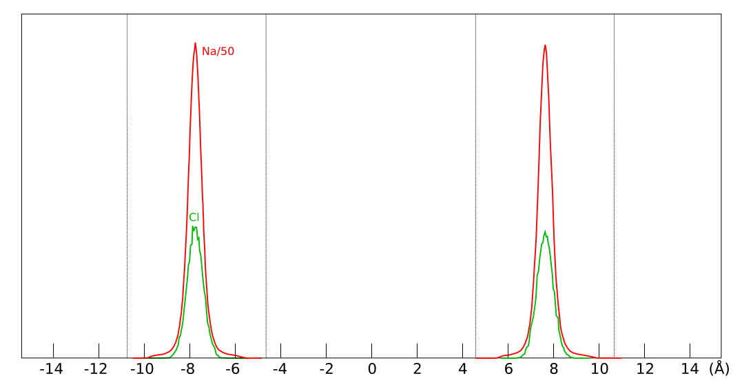
the exact same place within the clay, as shown here
This figure shows evaluated chloride density profiles in the direction perpendicular to the mineral layers in MD simulations of Na-montmorillonite (Hsi15) and Ca-montmorillonite (presented in the supporting information to Hsi22). While I have arbitrarily scaled the profiles along the y-axis in the above figure for visualization purposes, emphasis is here on the identical position within each interlayer. Note that the simulated system contains two separate interlayers, indicated by dotted vertical lines.5
One lesson from these results is that researchers who struggle with getting chloride to enter interlayers in their simulations could use CaCl2 rather than NaCl. At e.g. an external chloride concentration of \(\sim\)0.5 M, the amount chloride in the clay is about seven times larger in Ca- as compared with Na-montmorillonite, which substantially reduces the required convergence time for the simulation.
These results also highlight the urgent need for empirical data. As I
pleaded for when
concluding the assessment of chloride equilibrium concentrations in Na-bentonite, labs all over the place should routinely produce and
publish ion equilibrium measurements. It is certainly a failure of the
bentonite research field that no published empirical data exists that
can be used to compare with these theoretical results. Indeed, as far
as I’m aware, no published systematic empirical data exists at all,
for anion equilibrium concentrations in calcium dominated
bentonite.6
Note that the implication of the results discussed here is not simply
some noted interesting difference in chloride equilibrium in different
types of montmorillonite. Rather, as the results indicate that
montmorillonite interlayers play by the rules of ordinary Donnan
equilibrium, they are an additional blow to the entire contemporary
multi-porous model description of compacted water saturated bentonite.
Footnotes
[1] As I often nag about on this blog, it is quite silly to use complete anion exclusion as a starting point when studying compacted bentonite, and then trying to “confirm” such a notion with e.g. MD simulations. There is no rationale for this assumption in the first place; as we have discussed earlier, the idea seems to have originated from misunderstanding the Poisson-Boltzmann equation. Moreover, there is solid empirical evidence for salt entering interlayers, in particular from measured swelling pressure response.
[2] Hsiao and Hedström (2022) call this ratio a partition
coefficient, which complies with the scientific literature on
e.g. polymer membranes. As I discussed
here, I have chosen to stick with some of my own terminology. I
hope this does not cause unnecessary confusion.
[4] That the activity coefficient ratios do not depend strongly on external concentration in this concentration interval is also compatible with the mean salt approach that I have suggested to use for compacted bentonite. For the external solutions, mean salt activities varies quite little in this concentration range, and since the interlayer concentrations only vary with a few percent, it make sense to assume that the interlayer activity coefficients basically remain constant. Hsiao and Hedström (2022) actually note that the undulation pattern in the potential of mean force in the direction of the reaction coordinate is essentially independent of the external solution, and conclude that the interlayer environment is essentially independent of external conditions.
[5] The nearly
identical profiles within each interlayer is also a confirmation
that these simulations are properly converged.
[6] An indication that CaCl2 in Ca-montmorillonite behaves as discussed is found here.
Over a long period on the blog, we have systematically examined studies on chloride equilibrium in sodium dominated bentonite. We have now individually assessed each study that was deemed to have potential to provide relevant information. In this blog post we make some overall conclusions and give an updated picture of what is actually known empirically regarding chloride equilibrium in bentonite.
The assessment included seven studies, which are summarized in the table below. The table also provides links to each individual assessment.
These studies are the only ones, to my knowledge, that meet the
following criteria:
They involve chloride
There are both theoretical and empirical arguments for that different anions may have different equilibrium concentrations (for otherwise similar conditions). In the assessment it has therefore been important to stick to one and the same type of equilibrating anion. Moreover, chloride is certainly the anion that has been studied the most within bentonite research, with iodide as its closest “competitor”.
They involve sodium dominated bentonite
This include commercial products, such as “MX-80”, “Kunigel V1” or “Kunipia F”, or materials that were intentionally prepared for the study (more or less pure Na-montorillonite).
Some studies exist where ion equilibrium is explored in other systems, e.g. claystone or bentonites dominated by divalent counter-ions. But, since we have every reason to belive that the conditions for ion equilbrium are different in such systems, as compared to Na-bentonite, we must be careful not to include them in the analysis. We shouldn’t compare apples and oranges.
They have a specified external sodium solution
Without some knowledge of the composition of the solution in contact with the sample, an evaluated chloride concentration cannot be related to any relevant equilibrium condition. Furthermore, if the water chemistry of the equilibrating solution is too complex (e.g. involving several cations), the equilibrium cannot in a reasonably straghtforward manner be related to chloride concentrations in a sodium dominated system.
They have a systematic variation of either density or external background concentration or both
My main motivation for making these assessments is for using equilibrium data to better understand salt exclusion in bentonite. This can reasonably only be achieved if density and/or background concentration has been systematically varied.
In the following we will refer to each study with the identifying
label listed in the table above.
Comments
Through-diffusion is unneccesary
A majority of the examined studies are
through-diffusion studies (Mu88, Mo03, Vl07, Is08, Gl10). A
through-diffusion test set-up is, in fact, much more complex than
required for only studying equilibrium quantities: it involves
monitoring the chemical evolution of the external solutions (often
using radiochemical methods), and the final state (steady-state)
concentration profile is often extracted, by meticulously sectioning
and analyzing the sample (studies where final state profiles were
extracted are indicated by a “p” in the above table).
Additionally, extracting relevant information from flux data requires fitting a two-parameter model. In all assessed diffusion studies, one parameter relates to mobility (either an “effective” or an “apparent” diffusion coefficient) and one to ion equilibrium (“effective porosity”, “anion-accessible porosity”, or a “capacity factor”).1 Consequently, through-diffusion tests, despite their complexity, only provide indirect estimates of equilibrium concentrations, and the accuracy of the estimated parameters naturally depends on details of the fitting procedure and the sampled data. In this regard, most of the studies we have examined report inferior fitting procedures and flux data, where the transient stage of the process has not been adequately sampled (the only exception being Gl10).2 Estimated “effective porosities” are therefore not very reliable. This imprecision can sometimes be mitigated by also using information on the final state concentration profile. But this part of the analysis then essentially corresponds to making a quite complicated equilibrium test. Two of the five diffusion studies — Mu88 and Mo03 — were discarded because evaluated parameters (and the underlying data) are too uncertain.
From an ion equilibrium perspective, through-diffusion tests are
consequently not very “economical”.
The obvious alternative are straightforward equilibrium
tests, where samples simply are equilibrated with specified external
solutions. This can in principle be done without monitoring, and only
requires the patience to wait long enough. The lack of any requirement
to monitor these types of tests also makes them suitable, I imagine,
for involving many samples without significantly increasing the
experimental workload.
Most equilibrium tests have not been adequately performed
Although they are conceptually much simpler, only two of the assessed
studies are pure equilibrium tests (Mu04 and Mu07).
A third (Vl07) performed explicit equilibrium measurements
as part of a diffusion study.
Essentially all studies in the assessment that have recorded concentration profiles show interface excess, i.e. an increased amount of ions near the edges as compared with the interior of the samples. As this effect seems to be universal,3 it must be accounted for when making equilibrium tests, or evaluated concentrations will be overestimated. Doing this should be quite straightforward, by, for example, quickly sectioning off the first few millimeters on both sides of the samples during dismantling. Unfortunately, this has not been done in the assessed equilibrium studies,4 which makes them unsuitable. Vl07, on the other hand, recorded full profiles, and the excess effect was accounted for.
Relevant parameter ranges
After discarding two diffusion studies and two equilibrium studies,
only three studies remain for which the evaluated equilibrium
concentrations are deemed sufficiently accurate: Vl07, Is08 and Gl10.
But we should also consider the relevance of the chosen density and background concentration ranges — something that has not been discussed to any greater extent in the individual assessments. My main motivation for performing this assessment is for using equilibrium concentration data for testing models for salt exclusion in compacted bentonite. A full understanding of ion equilibrium in such systems is crucial for e.g. a relevant chemical description of bentonite buffers in radioactive waste repositories. Therefore, a preferred effective montmorillonite density range is approximately 1.2 — 1.7 g/cm3, say.
With also this criteria in mind, we may therefore rule out two of the three remaining studies; Is08 treats low density systems (\(<\) 1.0 g/cm3), and Gl10 only considers an extremely high high density (1.9 g/cm3).5 This leaves us with a single study that passes both the test of providing accurate data on chloride equilibrium concentrations and being measured in relevant parameter ranges: Vl07. This study covers the approximate density range 1.15 — 1.75 g/cm3, and concentration range 0.01 — 1.0 M.
A single relevant study
On the one hand, it is great news that we have verified some data as
actually useful for evaluating salt exclusion in compacted
bentonite. On the other hand, it is very unfortunate that there only
is one single study!
Moreover, although the results of Vl07 most definitely are useful, they are not optimal. A more “pragmatic” problem with this study is that it reports whole sets of “Cl-accessible porosities”1 for each sample tested, together with an average value. But these different values simply reflect the uncertainty of the parameter for individual samples. If the study had no issues (experimental or modeling related), these values should all be the same, as they are evaluated from one and the same sample. In our assessment we identified that the major part of this uncertainty stems from evaluations from diffusion modeling, while estimations made from equilibrium considerations are more robust (total out-diffusion and stable chloride content). It is thus these estimations in Vl07 that are deemed useful, while the diffusion estimations should be discarded. Note that, since “Cl-accessible porosities” estimated from flux data are sub-optimal, so are the reported average values.
Unfortunately,
severalstudies have
used or
reported
the Vl07 data (as well as other data we have assessed) without
sufficient rigor when evaluating salt exclusion in compacted
bentonite. As a relatively recent example of this,
Gimmi and Alt-Epping (2018) compare two models for chloride exclusion with empirical data
in a figure that looks very similar to this6
In addition to the VL07 data, this plot also compare with data from Mu886 — a study that we have discarded. Taking the above plot at face value it is hard not to wonder what use the experimental data really has — the spread at certain places is almost an order of magnitude (indicated in the figure). You can basically fit any favorite model to this data (or rather, you can fit no model to this data). Gimmi and Alt-Epping (2018) anyway compare the data with two Donnan equilibrium models. One (“full Donnan”) is essentially equivalent to the homogeneous mixture model (all pore space is treated equally), while the other includes several specific additional model components (“free” porosity, exchange “sites”). Gimmi and Alt-Epping (2018) use this plot to argue for that these particular additional components become significant for bentonite at the lower density. But if we “clean up” the plot and only use data points that has passed the present assessment, the picture is instead this
With this version of the data we can at least convince ourselves that
it obeys the rules for Donnan equilibrium. But I mean that it is hard
to draw any more detailed conclusions than that. In particular, it is
a hard stretch to believe that the suggested more complex model has
any particular significance.7
The Vl07 data also has the more fundamental problem that the detailed
ionic composition of the system is not fully controlled. This is
actually the case for all assessed studies that use “natural”
bentonite rather than specifically prepared homoionic clay, and
relates to to the presence of uncontrolled amounts of divalent
cations.
Problems with ignoring the detailed equilibrium conditions
When “natural” bentonites — which generally contain more than one
type of cation — are contacted with a pure sodium solution, it is
inevitable that the material and the solution begin exchanging
cations. Furthermore, since these materials contain accessory
minerals, dissolution/precipitation processes are most probably also
initiated. Thus, at the time when the equilibrium concentration is
recorded, the exact chemical conditions are typically not known. In
particular, it is not clear exactly what e.g. the Na/Ca ratio is in
the clay. To make issues worse, the extent of this effect depends
significantly on the concentration of the external solution, where we
expect a purer sodium clay for higher external concentrations. Since
the external concentration is often varied by orders of magnitude in
these studies, this implies that quanities evaluated at different
concentrations most likely correspond to slightly different systems
(e.g. clay samples with different Na/Ca ratios). Thus, even if we have
taken measures when selecting studies to not compare apples and
oranges, this problem partly remains.
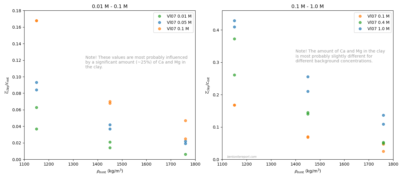
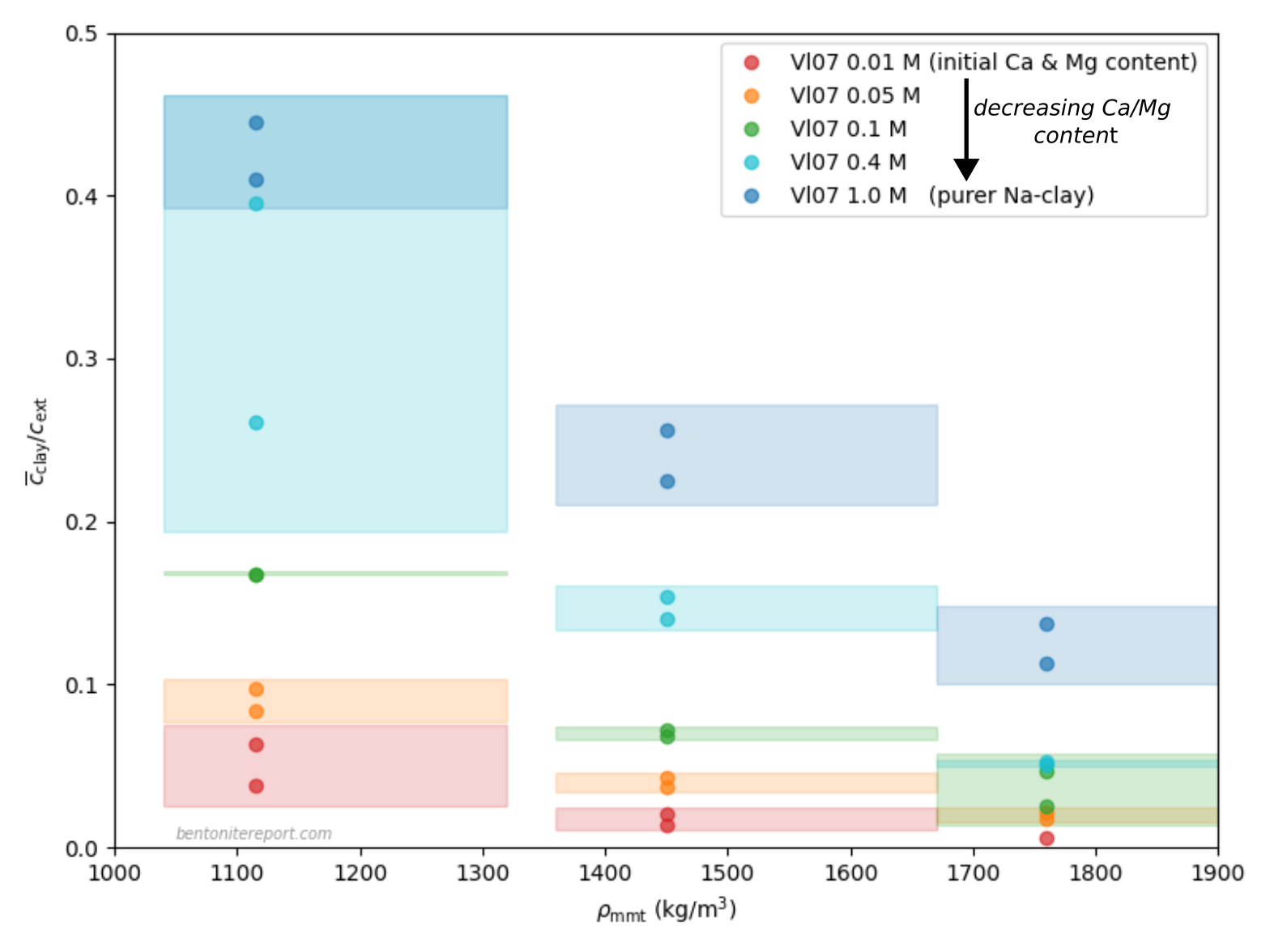
Relevant data for chloride equilibrium concentrations
Below is plotted the chloride equilibrium data that has been found
robust and relevant in the assessment (i.e. part of the data reported
in Vl07)
These values have been evaluated from the “Cl-accessible porosities” reported in table 6 in Vl07.8 The exact values of equilibrium concentration ratios and effective montmorillonite densities depend on adopted values for grain density and montmorillonite content. Here we have adopted \(\rho_s\) = 2800 kg/m3 and 80% montmorillonite. Note that equilibrium concentrations and densities are burdened with additional uncertainties that are not indicated in the above diagram. Note also that although most conditions in the above plot have two data points, these correspond to a single sample. For more details we refer to the individual assessment.
Comparing the above plot with
the one presented in the initial blog post on the assessment —
which included all available data — we note a considerably
less chaotic picture. At least, the robust Vl07 data gives evidence
for the two main features that we discussed in the initial blog post:
Chloride exclusion increases with increasing density at constant background concentration
Chloride exclusion decreases with increasing background concentration at constant density
It must be emphasized that the Vl07 data most probably has a
systematic “error”, in the sense that the data for lower background
concentrations (0.01 — 0.1 M) most probably is influenced by a
significant amount of divalent exchangable cations in the clay (Ca and
Mg). In contrast, for higher background concentrations (0.4 M, 1.0 M),
the clay is most probably in a purer sodium state.
A hundred labs should each make a hundred equilibrium tests!
After finishing this assessment the loudest question in my head is: why are not a hundred labs already on their way to each make a hundred equilibrium tests? Not only has the bentonite research sector failed when we must rely on a single soon 20-year-old study to have some idea of chloride equilibrium in sodium dominated bentonite. For other anions we essentially have no systematic data! As mentioned above, a general understanding of ion equilibrium is required in order to perform relevant chemical modeling of e.g. bentonite buffers in radioactive waste repositories.
[1] Here we do not discuss the
reasonability of these models and model parameters. I am, however,
arguing heavily in many
otherplaces on the blog that none of them are conceptually
sound. Here I have described how experimentally accessible equilibrium
concentrations can be extracted from “anion-accessible porosity”
parameters.
[2] This bad test design
isstillverycommon.
Through-diffusion tests should reasonably be designed so that the
outflux curve can be adequately sampled. As this curve behaves
drastically differently in the transient and in the steady-state
stages, the sampling frequency should reasonably be adapted.
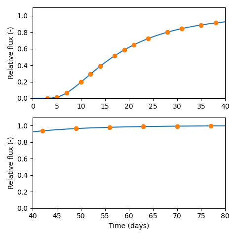
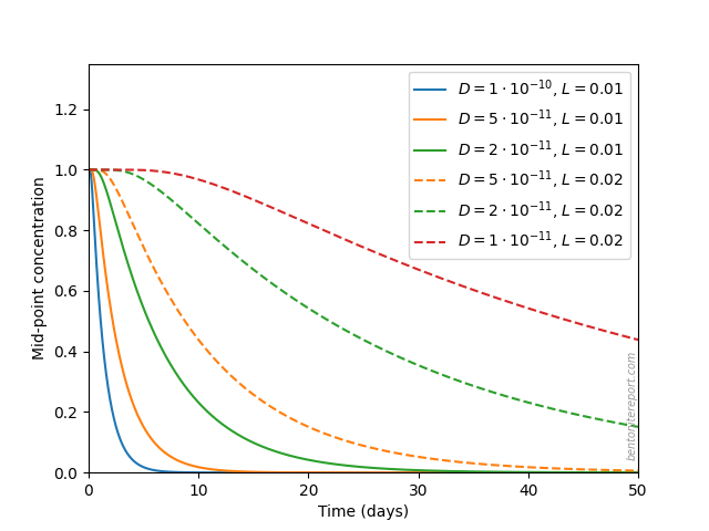
As an example, if a lab has the capacity to make measurements at most every second day (as is done in e.g. Vl07), I suggest starting diffusion tests on a Friday and design them so that essentially no tracers reaches the target reservoir during the weekend. This can be achieved by aiming for a breakthrough time of about 20 days. The breakthrough time is related to diffusivity (\(D\)) and sample length (\(L\)) as \begin{equation*} t_\mathrm{bt} = \frac{L^2}{6D} \end{equation*} Consequently, to keep \(t_\mathrm{bt}\) relatively constant, sample lengths should be adjusted depending on the expected value of the diffusivity. For a breakthrough time of 20 days, \(D = 10^{-10}\) m2/s corresponds to \(L=32\) mm, and \(D = 10^{-11}\) m2/s to \(L=10\) mm.
With a breakthrough time of about 20 days, and tests started on
Fridays, I suggest the following measurement protocol
3 times a week the first 3 weeks (Monday, Wednesday, Friday)
2 times a week the following 3 weeks (Monday, Friday)
1 time a week the following 5 weeks (Friday)
This would give sampling at 20 occasions over about 80 days that
ideally corresponds to four times the breakthrough time, like this
However, I further argue for that through-diffusion tests generally
should be avoided. Diffusivities are more conveniently (and quickly)
measured in closed-cell tests. Likewise, for equilibrium properties
it is obviously better to perform equilibrium
tests. Through-diffusion tests, in my opinion, are only motivated
under
particular circumstances, e.g. for making several non-destructive
measurements in the same sample under various conditions.
[3] I am fully convinced that this is an effect due to swelling during sample dismantling. Molera et al. (2003) and Glaus et al. (2011) have presented other interpretations, which we have briefly discussed in the assessments. I intend to write a future separate blog post on this topic.
[4] Sample
information in Mu07 is sparse and it is not clear how dismantling
has been performed, but nothing suggests that interface excess has
neither been identified nor handled. In the individual assessment of
this study I came to the conclusion that this data after all can be
useful for evaluating models for salt exclusion. Here I anyway
discard the results, mainly due to the above mentioned lack of
information. This data should be kept in mind, however.
[5] Both Is08 and Gl10 provide interesting information,
which should not be completely forgotten. In particular, Is08 report
results for extremely high background concentrations (5.0 M). Gl10,
on the other hand, show a dependency on background concentration of
the diffusivity not seen in other tests. I was not able to rule out
this effect as an artifact and therefore encourage the bentonite
research community to help clarify what is occurring in these
specific systems.
[6] The reference for
the points labeled “M89” in
Gimmi and Alt-Epping (2018) is Muurinen et al. (1988), i.e. Mu88. I have not changed the label,
however, because the plot contains more data than what is reported
in Mu88. I have not been able to identify the source for this
additional data. We may also note that the Vl07 data reported here
appears to be quite randomly chosen; for some systems are chosen
data evaluated from diffusion, for others, data evaluated from
equilibrium measurements.
[7] On the contrary, there are many additional arguments for that sodium bentonite at 1.3 g/cm3 does not contain significant amounts of “free” porosity. Moreover, in my head, the procedure of treating ion exchange with both a Donnan equilibrium model and a surface site sorption model can only lead to overparameterization problems. It is also unreasonable in this context to add conceptually completely different features before the “full Donnan” model is treated in full, e.g. by including activity corrections.
[8] One entry in that table, for stable chloride at 1.9 g/cm3 and background concentration 0.01 M, has been discarded. The table also appears to contain a couple of typos, which have been corrected.
Reading Gl10 gives the impression that the study consists solely of through-diffusion tests of a set of different tracers (HTO, sodium, chloride), in a set of different materials (Kaolinite, “Na-Illite”, Na-montmorillonite), at nominal density 1.9 g/cm3. A lot of additional information, however, is published in a later, completely separate publication: Glaus et al. (2011), which we will refer to as Gl11. Needless to say, this is a quite peculiar way of reporting a study. For instance, Gl10 do not provide any geometrical information about the samples (!), but this is found in Gl11; Gl11 also report corresponding out-diffusion measurements that apparently were made.1
Even with the combined sources of Gl10 and Gl11, information is not
entirely complete. For example, tests have been carried out in
duplicates, but evaluated diffusion parameters are only reported as
averages (table 2 in Gl10). Furthermore, the sources give
contradictory information in some instances (this is further discussed
below). Scraping both sources for information, these are the tests
that have been performed, as far as I understand:
Through-diffusion
In total 8 separate tests were performed, with NaClO4 background concentrations of 0.1 M, 0.5 M, 1.0 M and 2.0 M. These were performed in sequence in four different tests cells. Thus, two tests at 1.0 M background concentration were first performed in two different samples; thereafter, the same two samples were used for two additional tests at 2.0 M. Similarly, in two other samples, two 0.5 M tests were followed by two 0.1 M tests. The steady-state concentration profile in the clay was measured in one single test, performed at 0.1 M background concentration.
In this assessment we will also make use of the results from through-diffusion of water (HTO). These were made at background concentrations 0.1 M and 1.0 M. We will return to the question of whether they were carried out in the same samples as used for the chloride-diffusion experiments.
Out-diffusion
Most of the through-diffusion tests were followed by out-diffusion tests: after steady-state was reached, the external reservoirs were exchanged for tracer free solutions, and diffusion of chloride out of the sample was recorded.
Out-diffusion was tested on all samples at background concentrations 0.5 M and 2.0 M, and on one sample at background concentration 0.1 M.
Sorption
The montmorillonite material was tested for sorption of chloride, in suspensions with background concentrations of either perchlorate or chloride (at 0.5 M).
Equilibrium tests
At least one test was conducted to investigate the amount of ClO4 in the clay after the sample was equilibrated with a specified external concentration.
Investigation of swelling during dismantling.
The samples were cylindrical with diameter 2.54 cm, and with slightly different lengths, close to 1.0 cm. The sample volume is thus roughly 5 cm3.
In the following, we mainly refer to the chloride diffusion tests in
montmorillonite. Although the diffusion parameters are only reported
as averages, each individual parameter is actually found in a single
plot in Gl10 (“Fig. 6”). From this plot we can extract results from
each individual through-diffusion test (see below).
In Gl10 are also presented breakthrough curves (flux vs. time) for four tests, one for each different background concentration. Similarly, in Gl11 are presented three flux-vs.-time plots for out-diffusion. As will be further discussed below, we have to do some combined guess- and detective work in order to identify these flux evolution curves with specific samples.
Material
The material is referred to as montmorillonite “from Milos”, and was prepared specifically for the study. Bentonite from Milos (Greece), purchased from Süd-Chemie (now Clariant), was repeatedly washed in strong NaCl solutions to remove most of the accessory minerals and to convert the clay to essentially pure sodium-form. Excess NaCl was subsequently removed from the clay by dialysis. Gl10 present analyses of the chemical composition of both the used materials, as well as of a further purified 0.5 \(\mu\)m fraction of the montmorillonite material. From these analyses it is concluded that the used montmorillonite still contains some silica accessory minerals (3 — 4%), as well as some carbonate (calcite). We may thus assume a montmorillonite content of around 95%.
Concerning the cation population, Gl10 assert that the detected calcium is “most probably” present as CaCO3 rather than being part of the exchangeable cations. However, as the purification procedure used here is quite similar to that used in Muurinen et al. (2004) — that we have assessed earlier — we may expect some influence of calcium on the exchangeable cations. Muurinen et al. (2004) measured a Na/Ca-ratio of approximately 90/10 in their material, which also contained some carbonate (as well as sulfate). Here we assume that the used Na-montmorillonite is basically a pure sodium system, but should keep in mind that the presence of calcium may somewhat influence the results, especially since the different samples are exposed to very different external sodium concentrations.
Sample density
The nominal density for all samples appears to be 1.9 g/cm3, but actual sample densities are not reported (in Gl10, it is even hard to find information on nominal density). However, results of HTO diffusion in four tests (at 0.1 M and 1.0 M background concentration) indicate a considerably lower density. Porosities inferred from the breakthrough curves for these tests range between approximately 0.35 — 0.42. As is further discussed below, we here choose a range for the porosity of 0.321 — 0.394. Assuming a grain density of \(\rho_s\) = 2.8 g/cm3, this corresponds to a density range of 1.9 g/cm3 — 1.7 g/cm3 (effective montmorillonite density 1.87 g/cm3 — 1.66 g/cm3).
Uncertainty of external solutions
We have no reason to doubt the validity of the solutions used, and
will assume no uncertainty here.
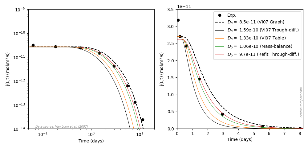
Evaluations from the diffusion tests
The chloride diffusion data in Gl10 and Gl11 is essentially analyzed in terms of the effective porosity model, although the fitted parameters are the “effective diffusivity” (\(D_e\)) and the “rock capacity factor” (\(\alpha\)). But for chloride, Gl10 use \(\alpha\) and \(\epsilon_\mathrm{eff}\) (the “effective porosity”) interchangeably.2 To avoid confusion, we will only use the notation \(\epsilon_\mathrm{eff}\).
As mentioned, Gl10 only tabulate the mean values of \(D_e\) and \(\epsilon_\mathrm{eff}\) for each background concentration, but we can extract each individual parameter graphically. The extracted \(D_e\) and \(\epsilon_\mathrm{eff}\) are listed here.3
With a single exception, the averages are identical with what is listed in table 2 in Gl10, which confirms the accuracy of the extracted parameters (for 1.0 M background concentration, the average \(\epsilon_\mathrm{eff}\) is 0.050 rather than the tabulated value 0.051). In the above table are also listed the corresponding pore diffusivities, evaluated as
From the flux and profile data found in Gl10 and Gl11, we can also
evaluate several pore diffusivites ourselves. Such values are
presented in the fifth column in the above table, and corresponding
steady-state fluxes are found in the sixth column. Below is compared
various flux vs. time data with my own simulations.
Regarding the breakthrough curves, the test design is here much better
than what we have encountered in earlier assessments; the transient
stage is properly sampled rather than that the data mainly represents
a sequence of steady-state measurements.4 This makes the inference of diffusion parameters
quite easy and robust.
Comparing the through-diffusion and out-diffusion results we can conclude that the data presented in Gl10 and Gl11 for background concentration 0.1 M most probably is for the same sample. Although the fitted parameters differ somewhat, the text of Gl11 states a steady state flux of 1.8⋅10-13 mol/s/m2 for the other 0.1 M sample, which was subsequently sectioned. As the presented through-diffusion flux is considerably smaller we may conclude that this is the same sample for which out-diffusion subsequently was conducted.
For the 0.5 M data, we can instead conclude that the two data sets must stem from two different samples, as the steady-state fluxes differ by roughly a factor of 2. For the 2.0 M data, the fitted parameters are very similar for the two test phases, which may indicate that they were measured in the same sample. However, the parameters are also very similar for the other test. The same is true for 1.0 M data (for which no out-diffusion was performed).
From steady-state fluxes and reported values of \(D_e\), we can calculate the corresponding tracer concentration in the source reservoir as
where \(L\) is sample length.5 Source tracer concentrations evaluated in this
way are presented in the last column in the above table (source
concentration is only reported for a single test, in Gl11).
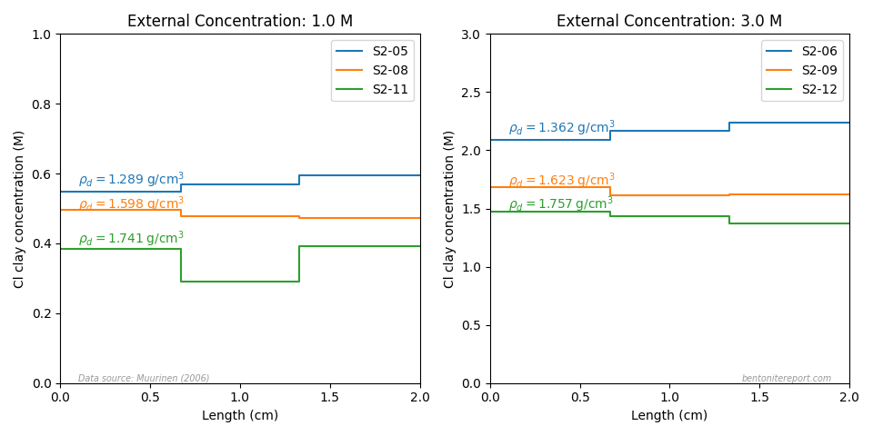
Finally, we can also look at the presented tracer profile at
termination, which was determined in a single case,6 for one of the 0.1 M tests.
We note — as does Gl11 — that the concentration profile shows quite extensive interface excess, a topic that we have discussed in a separate blog post. The main focus of Gl11 is actually a modeling treatment of these regions, but here we focus on the linear interior part of the profile.7 Fitting a line to this part (see figure) we extract a slope of -22.0 nmol/g/m. Gl11 do not report the corresponding density profile (that most certainly was measured), but using the nominal density (1.9 g/cm3), gives a corresponding clay concentration gradient of \(\nabla c_\mathrm{ss} = -0.0418\) mol/m4. Combining this value with the steady-state flux (1.8⋅10-13 mol/m2/s; reported in the text in Gl11), we can independently evaluate the pore diffusivity
This is in reasonable agreement with the value evaluated from \(D_e\) and \(\epsilon_\mathrm{eff}\).
In conclusion, even though crucial information is missing in Gl10, the re-evaluations made here, with help from information in Gl11, confirm the adequacy of the reported parameters \(D_e\) and \(\epsilon_\mathrm{eff}\). A perhaps single conspicuous detail is that the source concentration in one of the 0.5 M tests appears to have been about twice as large as for any of the other tests. There may, of course, be a reasonable explanation for this.
Evaluating chloride equilibrium concentrations
As noted in earlier assessments, the convenient quantity expressing the chloride equilibrium in through-diffusion tests is the ratio \(\bar{c}(0) / c^\mathrm{source}\), where \(\bar{c}(0)\) denotes the tracer concentration within the clay, at the interface to the source reservoir (for details, see here).
From the reported values of \(\epsilon_\mathrm{eff}\), the most
straightforward way to evaluate the chloride equilibrium
concentrations is
where \(\phi\) is the (physical) porosity. Gl10 (or Gl11) don’t provide information on actual measured densities, leaving us little choice but to use the nominal density in order to get a value for \(\phi\) in eq. 3. However, Gl10 also provide data for corresponding water (HTO) diffusion measurements. As mentioned above, these measurements indicate densities significantly lower than the nominal value. The (graphically extracted) values for \(D_e\) and \(\epsilon_\mathrm{eff}\) for HTO are
For water, the effective porosity parameter is really an estimate of
the physical porosity, and we can thus use this value to calculate a
corresponding density, which is presented in the last column in the
table.
Gl10 state
The diffusion of the various radioactive tracers (HTO, 22Na, 36Cl) was measured in sequence, each new tracer run was started after the out-diffusion of the previous tracer had been completed.
which is hard to interpret in any other way than that the above HTO parameters have been evaluated in the same samples in which chloride diffusion was tested. However, the protocol presented in Gl11 does not include any HTO diffusion “measured in sequence” (see above for information on the test protocol). The two sources evidently contain some contradictory information.8 Under any circumstance, as water diffusivity is claimed to be measured in samples with the same nominal density, we must assume a quite substantial uncertainty of the actual sample densities. In evaluating the chloride equilibrium concentrations, we therefore choose a porosity interval between the nominal value and the average given from the water parameters: \(\phi\sim\) 0.321 — 0.394. The table below lists the corresponding intervals for the chloride equilibrium concentrations
From the out-diffusion tests we can also evaluate the equilibrium concentrations “independently”, by integrating the flux. As discussed in the assessment of Van Loon et al. (2007), this integral (multiplied by sample area) gives one third of the total amount of tracers present in the clay at the start of the out-diffusion phase (these quantities are labelled “Acc.” in the above diagrams). With an estimate of the tracer concentration in the source reservoir, the equilibrium chloride concentration can thus be evaluated as
where \(N_\mathrm{right}\) denotes the final amount of tracers in the target reservoir. The corresponding chloride equilibrium concentrations are listed in the last column in the above table.
Finally, we also look at the 0.1 M test for which the steady-state tracer concentration profile was recorded. Extrapolating the linear part to the clay/source interface, gives a chloride content of 0.282 nmol/g, which corresponds to a clay concentration interval of 5.37⋅10-4 — 4.80⋅10-4 mol/m3, using the porosity interval defined above.9 Given the source concentration (0.024 mol/m3), these values correspond to a chloride equilibrium concentration ratio in the range 0.051 — 0.071.
The different ways of estimating chloride equilibrium concentrations provide a quite consistent picture (see above table). Although the information has been difficult to extract, it may thus seem that, in the end, all is good and well. However, we should note that the evaluated pore diffusivities show a quite peculiar dependency on background concentration.
Such a dependency, which has not been observed in earlier assessed studies, directly influence the evaluated equilibrium concentrations. As the breakthrough curves are so well sampled in the present study, this result can hardly be attributed to uncertainty in the values of \(D_p\). While Gl10 don’t explicitly identify this behavior (they do not evaluate \(D_p\)), a main focus of the study is actually to account for it, by means of “Archie’s law”, i.e. by suggesting a non-linear functional relationship between \(D_e\) and \(\epsilon_\mathrm{eff}\). I am strongly critical of such a treatment, but will refrain from discussing it here, as the focus of this assessment is the data itself rather than its interpretation (we have discussed this issue in a previous blog post).
An obvious alternative interpretation of this behavior is that chloride adsorbs on some system component, in the sense of becoming immobilized (what I have earlier dubbed true sorption). Gl11 test this hypothesis by performing additional batch sorption tests on the montmorillonite, in background solutions of NaCl and NaClO4 (0.5 M) at various pH. Although they cannot exclude a “\(R_d\)” value of the order of 10-4 m3/kg, they ultimately conclude that chloride do not sorb to any significant extent in these systems (and continues with “explaining” the behavior as resulting from other mechanisms).
I mean, however, that some experimental observations suggest that a sorption mechanism may be active. In addition to the above limit for the \(“R_d”\) value, we may note significant chloride sorption in the kaolinite samples, which were also studied in Gl10. There may of course be a reasonable explanation for why chloride sorption is observed in kaolinite, while it is not active in montmorillonite, but this issue is not really discussed in Gl10. Also, the recorded steady-state chloride content profile suggests a non-zero value at the interface to the target reservoir. This could, reasonably, indicate that some chloride is immobilized.
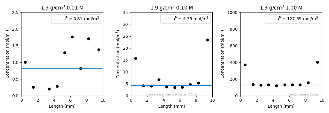
Perchlorate equilibrum concentrations
On the other hand, an additional argument against chloride sorption is that equilibrium perchlorate concentrations seem to be comparable with those evaluated for chloride. Gl11 don’t report perchlorate content directly, and we have to do some work to extract the corresponding equilibrium concentration in the 0.1 M sample that was sectioned. Gl11 plot the chloride tracer content for this sample together with “the concentration in the anion-accessible volume”, labelled \(c_\mathrm{acc}\).
\(c_\mathrm{acc}\) is, unsurprisingly, not a directly measured chloride concentration, but a quite elaborate interpretation of the data. From the unreported ClO4 content, an “anion-accessible porosity” variable has been calculated, by simply multiplying the physical porosity by the ratio between internal and external ClO4 concentrations. \(c_\mathrm{acc}\) is, in turn, defined as the actual measured chloride content distributed in a volume that corresponds to this “anion-accessible porosity”. By combining the reported chloride content (let’s call it \(\bar{n}_\mathrm{Cl}\)) and \(c_\mathrm{acc}\), we can thus de-derive the perchlorate equilibrium concentration as
Using this formula for the inner “linear” part of the profile (2 — 8 mm) gives the values 0.060, 0.059, 0.061 and 0.062, assuming nominal density. For porosity 0.394 the corresponding values are 0.044, 0.043, 0.044, and 0.045. We note that a range 0.043 — 0.062 for the equilibrium concentration ratio at 0.1 M background is in line with the previous evaluations. It should be noted, though, that this evaluation is for perchlorate, which not necessarily has the same equilibrium concentration as chloride. Nonetheless, this evaluation shows a similar, relatively high, equilibrium concentration also for this ion.
In fact, Gl11 provide results from yet another test where the focus is the perchlorate equilibrium,10 this time at a background concentration of 0.5 M. The results are reported as physical and “anion-accessible” porosities, evaluated from measuring water and perchlorate content.11
We note that also this sample shows substantial interface excess, but here we focus on the inner, relatively flat part (marked points in figure). From values of physical and effective porosity, we can directly calculate an equilibrium concentration in accordance with eq. 3. In this case the equilibrium concentration can also be related to a measured density. Using the average values gives a perchlorate equilibrium concentration ratio of \(\bar{c}_\mathrm{ClO_4}/0.5\; \mathrm{M} = 0.150\). Note that this value should be associated with density of 2.05 g/cm3 (the average porosity for the inner points is 0.259). This perchlorate equilibrium concentration ratio is nevertheless considerably larger than what was evaluated for chloride at (nominal) density 1.9 g/cm3 (0.11). This may indicate that perchlorate has a larger preference for the clay than chloride in these systems, but, as 2.05 g/cm3 is remarkably high, I suspect that measured water contents in this test have been systematically underestimated.
Summary and verdict
With only the information given in Gl10, I would judge the provided
information too uncertain to be used for quantitative process
understanding of chloride equilibrium in bentonite. With the
additional information provided in Gl11, however, we have seen that
the diffusion parameters — and consequently the equlibrium
concentrations that can be inferred — can be assessed to have been
quite robustly evaluated. Needless to say, access to a
completely separate publication should not be needed in order to make
this type of assessment. Nevertheless, my choice is to keep this data
to use for evaluating e.g. performance of models for salt exclusion.
A remaining uncertainty is the actual density of the tested samples. Results from corresponding water tracer tests suggest densities considerably lower than the nominal density. It not fully clear, however, if these water diffusion tests were conducted with separate samples or with the same samples as for the chloride diffusion tests.
Finally, these results complicate the picture of chloride equilibrium
concentrations in bentonite, as they do not fully comply with earlier
ones. In particular, here is observed a dependency of the pore
diffusivity on the background concentration, and chloride contents,
which are not seen in other studies. For anyone that is truly
interested in how salts distribute in bentonite, it should be a
priority to understand how the present results can be reconciled with
other chloride equilibirum results.12
Below is plotted the chloride equilibrium concentrations evaluated
from this study. For each background concentration is drawn an
“uncertainty box”, that takes into account the uncertainty in
density, as discussed above, and the corresponding interval in
equlilibrium concentration ratio. The corresponding points have been
arbitrarily put in the middle of these “uncertainty boxes”. The
effective montmorillonite density has been calculated assuming a
montmorillonite content of 95%.
To compare the present results with others, we have also plotted some chloride equilibrium concentration evaluated from Van Loon et al. (2007), that we have assessed previously.
[1] To be fair, reading Gl10 carefully, out-diffusion is briefly mentioned a couple of times.
[2] Gl10 rather use the term “accessible porosity”, and symbol \(\epsilon_\mathrm{acc}\), but we stick with the terminology that we have used in thepreviousassessments. Also, a critique of mixing the effective porosity model (that involves \(\epsilon_\mathrm{eff}\)) and the traditional diffusion-sorption model (that involves \(\alpha\)) is found here.
[3] For background concentration 0.5 M it is difficult to resolve if the diagram in Gl10 has a single point, or if there are two points on top of each other. As Gl10 claim that duplicates were made at all concentrations, here we have assumed two different samples with identical parameters.
[4] The
through-diffusion flux evolution for background concentration 0.1 M
plotted in Gl10 seems not to be complete: the diagram shows data
points up until day 160, but Gl11 state that the test was conducted
for 229 days.
[5] The simulations presented here use \(L\) = 9.75 mm for the samples with background concentration 2.0 M, and \(L\) = 10.25 mm for the samples with background concentrations 0.1 M and 0.5 M. These are average values from the sample lenghts reported in Gl11.
Tracer profiles of 36Cl in Na–mom were found to be in qualitative agreement with those found by Molera et al. (2003) and exhibited two distinct linear regions with different slopes. In contrast to Molera et al. (2003) we interpret the 36Cl profiles in terms of heterogeneities of compaction in the boundary zones of the clays and not as the result of two diffusion processes. In view of these ambiguities, tracer profiles were generally used as a consistency test and not for the calculation of \(D_e\) values.
At least to me, this way of writing gives the impression that
profiles were recorded for most of the tests. In Gl11, however, we
learn that only a single profile was recorded.
[7] Gl11 argue for that the non-linear
parts of the profile actually reflect the state of the sample during
steady-state, rather than being an effect of dismantling. I am
strongly critical to their arguments, and plan to comment on this in
a separate blog post.
[8] For the sodium measurements in montmorillonite, it is certain that the above statement is false. Most of these were made in 5.4 mm samples, and they were all sectioned. Morover, these were reported in a much earlier publication: Glaus et al. (2007).
[9] The clay concentration is calculated as \(\bar{c} = \bar{n} \cdot \rho_d/\phi\), where \(\bar{n}\) denotes the chloride concentration as amount per dry mass.
[10] The main focus in Gl11 is
actually the density distribution in the interface regions of the
sample, but this is a straightforward perchlorate equilibrium test.
[11] The data in
this plot has been “de-scaled”, as it was measured in a 5.4 mm
sample, but then “recalculated” (!?) for a 10 mm sample in Gl11.
[12] I intend to write a
follow-up blog post discussing these issues.
The study consists of chloride and iodide though-diffusion tests in sets of samples of “Kunigel V1” bentonite, mixed with either 0%, 30%, or 50% silica sand. Here we mainly focus on the chloride tests. Also, we exclude the samples with 50% sand, as the montmorillonite content is judged to small. For each type of material, chloride diffusion tests were performed with NaNO3 background concentrations 0.01 M, 0.5 M, and 5.0 M. All samples are cylindrical with diameter 2 cm and height 1 cm (giving a volume of 3.14 cm3) and have dry density 1.6 g/cm3, which means that the effective montmorillonite density varies in the different test sets. To refer to a single test we use the notation “sand mixture percentage/background concentration”, e.g. “30/0.5” refers to the test made on the sample with 30% sand and with background concentration 0.5 M.
A single additional test was performed on purified “Kunipia F” material, at dry density 0.9 g/cm3 and a background concentration of 5.0 M NaNO3. This density was chosen in order to have a similar effective montmorillonite dry density as the “Kunigel V1” samples with 30% sand.
All tests were performed at elevated pH in the external solution of 12.5 (initially), and the Cl diffusion tests were performed in a N2 glove box, with vanishing CO2 and O2 pressures. In total we here investigate 7 tests (of the 22 tests in the full study, we exclude 12 that concern iodide diffusion, and 3 that have 50% sand). In addition to the published article, these tests are also reported in a technical report (in Japanese).
Materials
“Kunigel V1” and “Kunipia-F” are simply
brandnames rather than materials specifically aimed for scientific
studies. This is similar to e.g. “MX-80” and “KWK”, that we have
encountered in
previousassessments.
I have found it rather difficult to obtain official data on “Kunigel V1” and “Kunipia F”; data sheets or technical specifications do not seem readily available online. Moreover, the Japan Atomic Energy Agency seem to contain their data within a database, and restrict its usage (this site seems a bit deserted, though). Fortunately, the open scientific literature contains some entries. These sources, however, provide quite different values for e.g. montmorillonite content and exchangeable cations in “Kunigel V1”.
Montmorillonite content
Several studies of “Kunigel V1” — including Is08 — refer to a single source for e.g. mineral content and cation exchange capacity: Ito et al. (1994),1 which states that “Kunigel V1” contains 46% — 49% montmorillonite. Other sources, however, claim considerably different numbers; e.g. Cai et al. (2024) states a montmorillonite content of 54.3%, while Kikuchi and Tanai (2005) states 59.3%.
Here, I do not intend to critically assess these various sources, but simply conclude that the montmorillonite content stated in Is08 must be viewed with some skepticism. The study they reference (Ito et al. (1993)) is significantly older than their own, and they do not indicate that they have investigated the material actually used. In this assessment we adopt an uncertainty for the montmorillonite content in “Kunigel V1” of 45% — 60%.
Concerning “Kunipia F” most sources I have investigated state a montmorillonite content above 99%, although some — including Is08 — set a lower limit at 95%. Here we assume that the montmorillonite content of “Kunipia F” lies in the interval 95% — 100%.
Cation population
Reports on cation exchange capacity (CEC) and exchangeable cations in “Kunigel V1” are also quite scattered in the scientific literature, as demonstrated in the table below.
CEC values (roughly) in the range 0.55 — 0.80 eq/kg are reported. These numbers will not be further assessed here, and we will assume an uncertainty of this range for the CEC in “Kunigel V1”.
One observation to be made is that some of the sources reporting relatively high CEC also reports relatively high montmorillonite content. The data from e.g. Kikuchi and Tanai (2005) gives an estimate of the cation exchange capacity for the montmorillonite of 0.75/0.593 eq./kg = 1.26 eq./kg, while the data from Ito et al. (1994) gives roughly 0.556/0.475 eq./kg = 1.17 eq./kg. These numbers are quite consistent and suggest that the reported differences in CEC may partly be due to differences in montmorillonite content in different batches of “Kunigel V1”.
We can further conclude that the reported amount of exchangeable sodium in “Kunigel V1” is rather stable (with some exception), while the amount of exchangeable calcium and magnesium scatter significantly. This scatter is mainly due to interference of soluble accessory minerals (see below; entries in the above table where such interference is obvious are put within parentheses). Thus, the exchangeable cation population in “Kunigel V1” can be estimated to about 80% — 90% sodium and about 10% — 20% di-valent ions (calcium and magnesium).
Some cation data for “Kunipia F” found in the literature is listed in the table below (the table contains a few entries for the variants “Kunipia-G” and “Kunipia-P”; these are indicated).
The most commonly reported CEC value in this little survey is 1.19 eq./kg, and I suspect that this has been supplied by the manufacturer (although the value 1.15 eq./kg has also been reported as a given from the manufacturer). As “Kunipia F” is mainly pure montmorillonite, note that this value (1.19) is consistent with the montmorillonite CEC estimated from “Kunigel V1” above. That being said, the scatter in reported CEC for “Kunipia F” is in the range 1.0 — 1.22 eq./kg.
The few reported cation populations of “Kunipia F” (and the variant “Kunipia G”, which is supposed to be identical in composition) that I have found have a higher sodium content as compared with “Kunigel V1”, roughly in the range 85% — 95%.
Soluble accessory minerals
Basically all sources I have encountered — including Is08 — say that “Kunigel V1” contains smaller amounts of calcite and dolomite. This is also quite evident from some of the reported results on exchangeable cations, where the sum of these substantially exceeds the evaluated CEC. Obviously, the presence of additional calcium and magnesium contribute to the uncertainty and complexity when evaluating effects of ion equilibrium in this material (just as for the cases of “MX-80” and “KWK”).
Sample density
The samples in Is08 were ultimately sectioned and analyzed (for the final state concentration gradient). Is08 nowhere state that they measured density of these sections. We thus proceed with using the nominal density of 1.6 g/cm3. Using the above estimated uncertainty in montmorillonite content we get the following intervals for the effective montmorillonite density
Samples
EMMD interval (g/cm3)
0% sand
1.05 — 1.24
30% sand
0.83 — 1.01
Kunipia F
0.87 — 0.90
Note that these intervals do not include uncertainty due to variation in density of the actual samples.
Uncertainty of external solutions
The samples were prepared by first saturating them with deionized water for more than two weeks, and thereafter contacting them with NaNO3 solutions for more than five weeks.
We have no reason to doubt the accuracy of the initial concentration of the salt solutions, but contacting a bentonite containing di-valent ions with pure sodium solutions inevitably initiates an ion exchange process. We have made the same conclusion for studies using “MX-80” and “KWK” bentonite. Similar to the previous studies, Is08 do not keep track of the exact chemical evolution of the external solutions, but we can calculate an estimate of the extent of the sodium-for-di-valent exchange.
The above diagram shows the result of equilibrating the specified amount of bentonite (3.14 cm3) with the specified amount of external solution (100 ml) for different initial NaNO3 concentrations. The calculation assumes that the bentonite only contains sodium and calcium, with an initial calcium content of 15%, a selectivity coefficient of 5 M, and a cation exchange capacity of of 0.65 eq/kg. The diagram shows the amount of calcium left in the sample after equilibration, as a function of initial NaNO3 concentration for the cases of 0% and 30% mixed-in silica sand. The dashed vertical lines indicate the external concentrations in the performed tests. We note — as we have done for several other studies — that the equilibrium amount of di-valent ions still in the bentonite depends significantly on the initial NaNO3 concentration: tests performed at 0.5 M and 5.0 M gives essentially a pure sodium clay, while samples used at 0.01 M still contain the initial 15% di-valent ions in the clay.
Since the “Kunipia F” material only is used in a test with background concentration of 5.0 M, we can quite safely assume that the exchangeable cation population in this particular test is basically 100% sodium.
It should be noted that the calculations have not accounted for the
additional di-valent ions present in the bentonite in form of
accessory minerals (calcite, dolomite). They thus probably
underestimate the amount di-valent ions still left in the clay after
equilibration.
Evaluations from the diffusion tests
The diffusion tests were performed by sandwiching the clay samples between a source and target reservoir of equal volumes, 50 ml. The initial Cl tracer concentration was 0.05 mM in the source reservoir, and 0.0 mM in the target reservoir.
The tracer concentration in both the source and target reservoirs were
periodically measured, but as far as I understand, none of the
reservoir solutions were replaced during a test. This means that a
certain concentration build-up occurs in the target reservoir, and
a corresponding concentration drop occurs in the source reservoir.
The test set-up furthermore involves quite wide “filter” components at the interfaces between clay and reservoirs.2 Is08 mean that these components restrict diffusion to such an extent that they must be included in the test analyses. With a rather complex set-up that involves evolving reservoir concentrations and “filter” influence, the preferred way to evaluate them would be a full simulation of the whole process. This is however not the procedure followed in Is08 (below we make such simulations).
Instead, Is08 center most of their evaluation around the measured steady-state flux,3 taking filter diffusion into account. In the blog post on on filter influence on through-diffusion tests we derived an expression for the steady-state flux, which can be written
where \(D_e\) is the effective diffusivity, and \(L\) the length of the clay
component. \(\Delta c_\mathrm{res}\) is the difference in
concentration between the two reservoirs, and \(\omega\) is the relative
filter resistance, given by
\begin{equation} w = \frac{2D_eL_f}{D_fL} \tag{2} \end{equation}
where \(D_f\) and \(L_f\) denote effective diffusivity and length of the
two confining “filters” (assumed identical).
which is the same expression as found in Is08 (eqs. 2 and 3 in Is08).
\(D_e\) is thus evaluated in Is08 by measuring \(j^\mathrm{ss}\) and \(D_f\), estimating \(\Delta c_\mathrm{res}\), and knowing the lengths of the clay and filter components (\(L\) = 1 cm, \(L_f\) = 1.5 cm). Note that this is a quite involved procedure, necessitated by the test design: the source reservoir is small enough for the concentration to significantly drop during the course of a test; the target is not replaced during the course of a test, resulting in an increasing concentration significantly different from zero; the sample is sandwiched between wide “filter” components; and, as far as I can tell, the external solutions are not stirred or circulated. With a simpler test design, the reservoir concentration difference could have been kept effectively constant, and influence from confining filters could have been avoided (the only case, really, where filter influence is unavoidable is for cation through-diffusion at low ionic strength). With this being said, a re-evaluation of the results demonstrates that the “filter” influence, after all, is quite moderate. We will further discuss this below.
Is08 estimate \(\Delta c_\mathrm{res}\) by using the average source reservoir concentration during the course of a test (\(\bar{c}_\mathrm{source}\)), and by assuming zero target reservoir concentration, i.e. \(\Delta c_\mathrm{res} = 0-\bar{c}_\mathrm{source}\). I do not really understand this, because the target reservoir concentration is clearly not zero; since the two reservoirs have the same volume it seems more reasonable to assume that the concentration drop in the source reservoir corresponds to an equal concentration increase in the target reservoir.4
The “filter” diffusivities are claimed to be measured in separate tests without clay components, but the reported values does not make full sense to me. It is claimed that three different values for \(D_f\) were used for the three different background concentrations. But we do not expect any significant difference in diffusivity due to background concentration. Does this mean that tests performed at a specific background concetration all used the same test cell, while different test cells were used for different background concentrations? Furthermore, the specified values are \(D_f = 3\cdot 10^{-10}\) m2/s for background concentration 0.01 M, \(D_f = 2.6\cdot 10^{-9}\) m2/s for background concentration 0.5 M, and \(D_f = 1.8\cdot 10^{-9}\) m2/s for background concentration 5.0 M. The \(D_f\) values at high background concentration are thus not only almost an order of magnitude higher than that for 0.01 M background, these values also implies a diffusivity larger than for pure bulk water.5
If we anyway use these values for \(D_f\) to calculate the relative filter resistances (eq. 2) we get maximum values for \(\omega\) of 0.077, 0.037, and 0.055 for background concentrations 0.01 M, 0.5 M, and 5.0 M, respectively (anticipating the evaluated \(D_e\) values in table 1 in Is08). These values are tiny, showing that their own estimations indicate insignificant “filter” influence.
In the following we de-derive the values for \(j^\mathrm{ss}\) and \(\Delta c_\mathrm{b}\) (the final clay concentration difference) used for evaluating the reported values of \(D_e\), “\(D_a\)”, and \(\epsilon_\mathrm{eff}\),6 and compare them with the raw flux and concentration profile data (available for the tests performed with 30% sand mixture).
Steady-state fluxes
The steady-state fluxes are nowhere stated explicitly in Is08, but it is straightforward to read them off from the provided “breakthrough curves”. To check the consistency of the reported parameters we may use these values and the reported values for \(D_f\) and \(D_e\) to back-calculate \(\Delta c_\mathrm{res}\) using eq. 3.
In this table are also listed the “expected” values of of the reservoir concentration differences, \(\Delta c_\mathrm{res,ex}\), estimated from subtracting the average concentration increase in the target reservoir from from 0.05 mM. We see that the reported values of \(D_e\) “overestimates” \(\Delta c_\mathrm{res}\) by 8% — 40%.
We do not have more information to assess whether this mismatch is
due to some actual inconsistency in the reported values or if it indicates
that the concentration difference stated in the article was not
actually what was achieved in the experiment. In any case, this is low
quality scientific reporting.
Concentration profile gradients
We can, however, continue by also checking the consistency of the estimated pore diffusivity, \(D_p\),7 which was evaluated by measuring the concentration gradient in the clay at the termination of the tests (\(\Delta c_b/L\)).8
The concentration gradients are not explicitly stated in the article, but we can read them off from the published concentration plots. By using the tabulated values of \(D_p\) we can use eq. 4 to back-calculate what values for the steady-state flux was used for their evaluation.
Note that some of these values of \(j^\mathrm{ss}\) are smaller than
what can be read off from the “breakthrough curves”. In particular,
the value for the 30/5.0 test is reduced by more than 30%. If we use
these values of \(j^\mathrm{ss}\) to re-calculate the corresponding
reservoir concentration differences, we get
Although the calculated value for \(\Delta c_\mathrm{res}\) still is larger than 0.05 mM for the 30/0.5 test, these values are now generally in better agreement with the “expected” estimations.
I do not really know what to make of these results. For the 30/0.01 and 30/0.5 tests, the slightly different results perhaps reflect the uncertainty in the estimation of \(j^\mathrm{ss}\) and \(\Delta c_b\). But there is clearly something wrong with the evaluation of the 30/5.0 test. From the diagram (fig. 2 in Is08), it is, for example, clear that this test has the largest flux.
Chloride equilibrium concentrations
The chloride equilibrium concentration is evaluated in Is08 in terms of an “effective porosity,”6 \(\epsilon_\mathrm{eff} = D_e / D_p\). But from eq. 3 and eq. 4 we see that it is really evaluated from
Note that the factors \(j^\mathrm{ss}L\) cancel; the evaluation of \(\epsilon_\mathrm{eff}\) is therefore less sensitive to the estimation of \(j^\mathrm{ss}\) (the flux only appear in the correction term due to filter influence). Thus, even if the evaluation of \(j^\mathrm{ss}\) evidently has its flaws, the evaluation or \(\epsilon_\mathrm{eff}\) is more robust. This reflects the fact that the equilibrium concentration, as the name suggest, does not depend on transport quantities; as is clear from eq. 5, \(\epsilon_\mathrm{eff}\) is simply an interpretation of the clay concentration (\(c_b\)). We have discussed this issue severaltimesbefore.
Eq. 5 also shows that the uncertainty in estimating the equilibrium concentration (or \(\epsilon_\mathrm{eff}\)) mainly stem from uncertainties in \(\Delta c_\mathrm{res}\), and uncertainty stemming from filter resistance (\(2j^\mathrm{ss}L_f/D_f\)). Both of these uncertainties could have been avoided with a better test design — if filter resistance was avoided, and if the source and target reservoirs were kept at (virtually) constant concentrations, the equilibrium concentration would be given directly from the clay concentration profile.9
One way to estimate the effects of these uncertainties is to simply
compare the reported values for \(\epsilon_\mathrm{eff}\) with the ratio
\(\Delta c_b/\Delta c_\mathrm{res,init}\), where
\(\Delta c_\mathrm{res,init}\) = -0.05 mM is the initial reservoir
concentration difference.
The differences are not that great, demonstrating that reported values
of equilibrium concentrations (\(\epsilon_\mathrm{eff}\)) are quite
robust, even though we have found inconsistencies in the underlying
transport quantities.
Why not just simulate the whole thing?
A better way, in my view, to extract the equilibrium concentrations from this rather complex test set-up is to simulate the tests completely. This is done here, taking into account the external reservoir, the “filter” components and using the homogeneous mixture model for the bentonite component. Note that the homogeneous mixture and the effective porosity models are equivalent when it comes to modeling this type of diffusion: the effective porosity parameter can be calculated from \(\epsilon_\mathrm{eff} = \phi\cdot\Xi\), where \(\phi\) is the physical porosity and \(\Xi\) is the ion equilibrium coefficient. Similarly, the diffusion coefficient in the homogeneous mixture model (\(D_c\)) can in this case directly be identified with the pore diffusivity in the effective porosity model (\(D_p\)). In these simulations we used \(\Xi\) and \(D_c\) as fitting parameters.
The fitted parameters are listed in the table below and compared to
the reported values of \(D_p\) and \(\epsilon_\mathrm{eff}\).
Test
\(D_c\) (10-10 m2/s)
\(D_p\) (10-10 m2/s)
\(\Xi\)
\(\phi\cdot\Xi\)
\(\epsilon_\mathrm{eff}\)
30/0.01
2.14
1.8
0.103
0.043
0.043
30/0.5
2.50
2.4
0.457
0.19
0.13
30/5.0
2.39
1.6
0.625
0.26
0.21
Below is the simulated outflux curves and final state clay concentration profiles compared with experimental data.
0.01 M background concentration:
0.5 M background concentration:
5.0 M background concentration:
The simulations were performed both with (green lines) and without
(red lines) including filters. It may be noted that both models can be
fitted equally well, confirming that filter effects are after all
small in these tests. Also, although the diffusion parameters change
to some extent, the fitted ion equilibrium coefficients are
essentially the same regardless of whether filters are included or
not. We note that the spread in the values for the diffusion parameter
is smaller for the simulations as compared with the reported
values. As we expect similar diffusivity in these identically prepared
samples, I see this as a confirmation that a simulation better
captures the experimental parameters. Concerning the ion equilibrium,
or equivalently the “effective porosity”, we note that the
simulations provide somewhat higher values as compared with the
reported quantities, both for test 30/0.5 and test 30/5.0. The values
are however still comparable, again demonstrating that they have been
more robustly extracted.
Summary and verdict
We have seen that Is08 has several flaws and weaknesses: the test design is unnecessarily complex, and from the provided data on clay concentrations and fluxes, we have noted inconsistencies, e.g. in the values adopted for the steady state flux. It is also not completely clear if the actual initial concentration differences between the external reservoirs is 0.05 mM (as stated in the article) or if this is some measured but not reported quantity. We have also noted that the material used (primarily “Kunigel V1”) suffers from several uncertainties in its composition.
All of these factors lead to uncertainty in the quantities we are primarily interested in, i.e. chloride equilibrium concentrations. We have also seen, however, that we have reason to believe that these reported quantities are considerably more robust; most simplistically, the equilibrium concentration can be inferred by extrapolating the clay concentration profile to the interface on the target side and comparing that value to 0.05 mM.
My choice is therefore to keep these values to use for evaluating e.g. performance of models for salt exclusion. One reason that this data is interesting for this purpose is the measurement of equilibrium concentrations at an exceptionally high background concentration.
Below is a diagram that summarizes the findings of this assessment.
This figure includes gray stripes to indicate the estimated uncertainty in effective montmorillonite density (for these tests we have no means to estimate the uncertainty of the reported equilibrium concentration). For two of the tests that we have been able to look at in more detail (30/0.5 and 30/5.0) we have added an “area of uncertainty” that both include uncertainty in density and concentration. The estimation of the uncertainty in concentration is here simply done by including the values inferred from completely simulating these tests. These “areas” are no formal confidence intervals, but should be viewed as giving a hint of the uncertainties involved.
[1] Is08 actually refer to a corresponding technical report, from 1993.
[2] Apart from
“real” filters, the sample is also confined by two thick
perforated components; the total “filter” length is specified as
1.5 cm!
[3] As the concentration continually
changes in the reservoirs this is not a true steady-state, but what
we could call a “quasi”-steady state (it is still easily
distinguished from the initial part of a through diffusion test).
[4] With reservation for that the target is consumed
due to quite frequent sampling — but this would contribute to an
additional increase of the target concentration.
[5] Note that these are effective diffusivities, and includes “filter” porosity (we are not told their values, but they can of course not be larger than unity). The only value of \(D_f\) that seems reasonable is the one for 0.01 M, which corresponds to a geometric factor of 6.7. To make things even stranger, for iodide the same value is used for \(D_f\) regardless of background concentration (\(3.9\cdot 10^{-10}\) m2/s).
[6] Is08 refer to this quantity as \(\alpha\), “the capacity factor”. But it is clear from the text that it is interpreted as an effective porosity, and we will therefore use the notation \(\epsilon_\mathrm{eff}\), in accordance with earlier assessments. Is08 actually also relate the parameter \(\alpha\) to sorption via the relation \(\alpha = \phi + \rho K_d\) (their eq. 6). This is however a mix-up of two incompatible models, which I have commented on here. We also note that Is08 actually never use the distribution coefficient, \(K_d\), for anything in their analysis.
[7] Is08 call this quantity \(D_a\), but it is not an “apparent” diffusivity, and I do not accept using this bizarre nomenclature. I will call the corresponding parameter \(D_p\) in accordance with e.g. the effective porosity model.
[8] Is08 define the clay concentration, \(c_b\), in terms of total clay volume. Alternatively it can be defined in terms of total amount of water, the difference being a porosity factor.
[9] Or, rather, chloride equilibrium concentrations can then be inferred directly from the value of the clay concentration profile at the interface to the source reservoir.
Mu07 actually report 9 more data points, but these originate from Muurinen et al. (2004) (which we have already assessed). This is not fully acknowledged in Mu07, but below I try to sort out the status of all data presented. We refer to Muurinen et al. (2004) as Mu04.
In similarity to Mu04, Mu07 is an equilibrium study (i.e. not a diffusion study) performed on purified “MX-80” bentonite. One of the main objectives in Mu07 is to investigate possible influence of sample preparation on the chloride equilibrium concentrations. The samples in Mu07 cover a large density range (0.6 — 1.5 g/cm3), but were all equilibrated with a single type of solution: 0.1 M NaCl.
Originally conducted and already reported tests
Mu07 state that the study is a continuation of the investigations
presented in Mu04 and present data on five different sets of samples,
prepared and equilibrated using different methods (labeled A —
E). What is not explicitly stated — but what is obvious if comparing
tables 1 and 2 in Mu04 with table 1 in Mu07 — is that sample sets D
and E are the same as previously reported in Mu04.
I find this quite remarkable, since two of these samples were
dismissed as “not reliable” in Mu04
(In my
assessment, I dismissed all tests in Mu04); here the same results
— which show an increase in equilibrium chloride content with
density — are not only re-reported, but modeled! The authors don’t
even seem aware that they have previously discarded the samples,
writing: “Surprisingly, it seems that the concentrations in the
sample types D and E start to increase at the highest
densities“. Furthermore, one of the (previously reported) data points
of sample set E, which have a clay concentration larger than
the corresponding concentration of the equilibrating solution, is
not included in Mu07. Needless to say, excluding data points
without motivation, or including previously discarded data is not good
scientific practice.
As the sample overview table in Mu07 also has some misprints,1 I here present a (hopefully) correct version that also indicates original publication (for the indicated sample-IDs, see the assessment of Mu04).
Type
Density (g/cm3)
Time d.w. (days)
Time 0.1 M (days)
Clay conc. (mM)
origin/remark
A
0.625
18+35
217
37
Mu07
A
0.812
18+35
217
29
Mu07
A
1.200
18+35
217
20
Mu07
B
0.670
222
107
35
Mu07
B
0.937
222
107
23
Mu07
B
1.389
222
107
15
Mu07
C
0.622
30
36
48
Mu07
C
0.731
30
36
30
Mu07
C
1.113
30
36
17
Mu07
C
1.382
30
36
14
Mu07
C
1.517
30
36
12
Mu07
D
0.754
0
40
65
Mu04 (S2-02)
D
0.855
0
40
39
Mu04 (S2-21)
D
1.273
0
36
22
Mu04 (S2-04)
D
1.636
0
36
24
Mu04 (S2-17; deemed “not reliable” in Mu04)
D
1.764
0
85
48
Mu04 (S2-18; deemed “not reliable” in Mu04)
E
0.750
0
12(?)
109
Mu04 (not included!)
E
0.875
0
12
61
Mu04
E
1.225
0
12
25
Mu04
E
1.516
0
12
12
Mu04
E
1.543
0
12
14
Mu04
In the following, the focus is solely on samples sets A — C (as
mentioned, the others have already been
assessed).
Material
The material appear to be the same as used in Mu04. I therefore refer to the assessment of that study for a detailed discussion. In brief, the material is purified “MX-80” bentonite, with a montmorillonite content above 90% and about 90% sodium as exchangeable cation.
Samples
Samples in the three different sample sets A — C were prepared in different ways. For set A, the clay was initially dispersed in deionized water at quite low density. After an equilibration time of 18 days (which included ultrasound treatment), the dispersion was slowly squeezed to achieve the intended densities. This squeezing phase lasted 35 days, after which the samples were contacted with 0.1 M NaCl and equilibrated for 217 days.
Samples in set B were prepared in the same type of sample holder as
those in set A, but the bentonite powder was directly compacted to the
desired density, and the samples were water saturated by contact with
deionized water for 222 days (!). Thereafter, the samples were
contacted with 0.1 M NaCl and equilibrated for 107 days.
The external solution was not circulated in the preparation of samples
in sets A and B. In contrast, samples in set C were prepared in cells
with external circulation. The bentonite powder was directly
compacted to the desired density, and the samples were water
saturated by contact with (circulating) deionized water for 30
days. The samples were then equilibrated with (circulating) 0.1 M NaCl
solution for 36 days.
Even if the preparation protocols are described quite detailed in Mu07, we are not given any information on sample geometry. We are not even told if the samples have the same geometry! (Given that they were prepared in different types of equipment, different geometries may certainly be the case.) Without knowledge on e.g. the characteristic diffusion lengths, it is impossible to assess e.g. whether the adopted equilibration times are adequate. Reasonably, the size of the samples are on the cm scale, and since the equilibration times are very long, we can guess that they have had time to equilibrate. This is in contrast to the samples in Mu04, which we have reason to suspect have not been completely equilibrated, as discussed in the assessment of that study. (Note that these samples are included in Mu07, as sample sets D and E.)
Mu07 does not provide any information on how sample density was
measured. Since we neither know the dimensions of the samples it is
therefore impossible to estimate any uncertainty of the reported
densities.
Chloride equilibrium concentrations
The following plot summarizes the reported chloride equilibrium
concentrations and corresponding densities in sample sets A — C.
Although the data show some significant scatter (e.g. for the two
lowest densities in sample set C), the main impression is that the
three different ways of preparing and equilibrating samples result in
quite similar values for the chloride equilibrium concentrations. Thus,
even if we know little about the samples, this coherence in the
results indicates that they have been properly equilibrated.
Possible interface excess salt
As we have discussed in
severalpreviousblog
posts, when performing equilibrium tests it is important to handle
the possibility that the samples have an increased salt content in the
interface regions. In the assessment of Mu04, my guess was that the
samples had not been handled specifically to deal with this possible
measuring artifact, and I neither see any reason to believe that this
issue has been addressed in sample sets A — C (we can, however, rule
out that too much salt entered these samples during saturation, since
deionized water was used in this phase).
The possible influence of interface excess depends, apart from general
sample treatment, on e.g. sample thickness and the concentration of
the equilibrating external solution. As noted above, we have no
information on sample thickness, but the external concentration is in
this regard quite low (we showed in an earlier post that the problem
of interface excess salt becomes more severe for thin samples and low
external concentrations). Therefore, we can certainly not exclude the
possibility that the reported equilibrium concentrations are
systematically overestimated due to possible influence of an interface
excess, especially for the denser samples (see
here for details on this).
An argument against that interface excess has significantly influenced
the results is the similar result for the three different sample
sets. Of course, this depends on how similar (or dissimilar) the
samples in the different sets are, of which we have no
information. Under any circumstance, it is very clear that Mu07
provides too little information to fully rely on the reported values.
Summary and verdict
From one perspective, Mu07 is a very straightforward study: samples of
purified bentonite (almost pure Na-montmorillonite) at various density
have been equilibrated with a single type of external solution (0.1 M
NaCl). The results also look reasonably coherent. However, the paper
contains way too little information on e.g. sample geometry and how
density and concentration were measured to fully rely on the
results. In particular, we cannot rule out a systematic overestimation
due to influence of interface excess salt. Furthermore, the main
reason to believe that equilibrium was achieved, is the
similarity between the different test sets.
My decision, however, is to keep these result to use e.g. for possible
qualitative process understanding (specifically, chloride exclusion).
But I will certainly keep in mind the quite extensive lack of
information associated with this data.
Vl07 is centered around a set of through-diffusion tests in “KWK” bentonite samples of nominal dry densities 1.3 g/cm3, 1.6 g/cm3, and 1.9 g/cm3. For each density, chloride tracer diffusion tests were conducted with NaCl background concentrations 0.01 M, 0.05 M, 0.1 M, 0.4 M, and 1.0 M. In total, 15 samples were tested. The samples are cylindrical with diameter 2.54 cm and height 1 cm, giving an approximate volume of 5 cm3. We refer to a specific test or sample using the nomenclature “nominal density/external concentration”, e.g. the sample of density 1.6 g/cm3 contacted with 0.1 M is labeled “1.6/0.1”.
After maintaining steady-state, the external solutions were replaced
with tracer-free solutions (with the same background concentration),
and tracers in the samples were allowed to diffuse out. In this way,
the total tracer amount in the samples at steady-state was
estimated. For tests with background concentrations 0.01 M, 0.1 M, and
1.0 M, the outflux was monitored in some detail, giving more
information on the diffusion process. After finalizing the tests, the
samples were sectioned and analyzed for stable (non-tracer)
chloride. In summary, the tests were performed in the following
sequence
Saturation stage
Through-diffusion stage
Transient phase
Steady-state phase
Out-diffusion stage
Sectioning
Uncertainty of samples
The used bentonite material is referred to as “Volclay KWK”. Similar to “MX-80”, “KWK” is just a brand name (it seems to be used mainly in wine and juice production). In contrast to “MX-80”, “KWK” has been used in only a fewresearchstudies related to radioactive waste storage. Of the studies I’m aware, only Vejsada et al. (2006) provide some information relevant here.1
Vl07 state that “KWK” is similar to “MX-80” and present a table with chemical composition and exchangeable cation population of the bulk material. As the chemical composition in this table is identical to what is found in various “technical data sheets”, we conclude that it does not refer to independent measurements on the actual material used (but no references are provided). I have not been able to track down an exact origin of the stated exchangeable cation population, but the article gives no indication that these are original measurements (and gives no reference). I have found a specification of “Volclay bentonite” in this report from 1978(!) that states similar numbers (this document also confirms that “MX-80” and “KWK” are supposed to be the same type of material, the main difference being grain size distribution). We assume that exchangeable cations have not been determined explicitly for the material used in Vl07.
In a second table, Vl07 present a mineral composition of “KWK”, which I assume has been determined as part of the study. But this is not fully clear, as the only comment in the text is that the composition was “determined by XRD-analysis”. The impression I get from the short material description in Vl07 is that they rely on that the material is basically the same as “MX-80” (whatever that is).
Montmorillonite content
Vl07 state a smectite content of about 70%. Vejsada et al. (2006), on the other hand, state a smectite content of 90%, which is also stated in the 1978 specification of “Volclay bentonite”. Note that 70% is lower and 90% is higher than any reported montmorillonite content in “MX-80”. Regardless whether or not Vl07 themselves determined the mineral content, I’d say that the lack of information here must be considered when estimating an uncertainty on the amount of montmorillonite (“smectite”) in the used material. If we also consider the claim that “KWK” is similar to “MX-80”, which has a documented montmorillonite content in the range 75 — 85%, an uncertainty range for “KWK” of 70 — 90% is perhaps “reasonable”.
Cation population
Vl07 state that the amount exchangeable sodium is in the range 0.60 — 0.65 eq/kg, calcium is in the range 0.1 — 0.3 eq/kg, and magnesium is in the range 0.05 — 0.2 eq/kg. They also state a cation exchange capacity in the range 0.76 — 1.2 eq/kg, which seems to have been obtained from just summing the lower and upper limits, respectively, for each individual cation. If the material is supposed to be similar to “MX-80”, however, it should have a cation exchange capacity in the lower regions of this range. Also, Vejsada et al. (2006) state a cation exchange capacity of 0.81 eq/kg. We therefore assume a cation exchange capacity in the range 0.76 — 0.81, with at least 20% exchangeable divalent ions.
Soluble accessory minerals
According to Vl07, “KWK” contains substantial amounts of accessory carbonate minerals (mainly calcite), and Vejsada et al. (2006) also state that the material contains calcite. The large spread in calcium and magnesium content reported for exchangeable cations can furthermore be interpreted as an artifact due to dissolving calcium- and magnesium minerals during the measurement of exchangeable cations (but we have no information on this measurement). Vl07 and Vejsada et al. (2006) do not state any presence of gypsum, which otherwise is well documented in “MX-80”. I do not take this as evidence for “KWK” being gypsum free, but rather as an indication of the uncertainty of the composition (the 1978 specification mentions gypsum).
Sample density
Vl07 don’t report measured sample densities (the samples are ultimately sectioned into small pieces), but estimate density from the water uptake in the saturation stage. The reported average porosity intervals are 0.504 — 0.544 for the 1.3 g/cm3 samples, 0.380 — 0.426 for the 1.6 g/cm3 samples, and 0.281 — 0.321 for the 1.9 g/cm3 samples. Combining these values with the estimated interval for montmorillonite content, we can derive an interval for the effective montmorillonite dry density by combining extreme values. The result is (assuming grain density 2.8 g/cm3, adopted in Vl07).
Sample density (g/cm3)
EMDD interval (g/cm3)
1.3
1.04 — 1.32
1.6
1.36 — 1.67
1.9
1.67 — 1.95
These intervals must not be taken as quantitative estimates, but as giving an idea of the uncertainty.
Uncertainty of external solutions
Samples were water saturated by first contacting them from one side with the appropriate background solution (NaCl). From the picture in the article, we assume that this solution volume is 200 ml. After about one month, the samples were contacted with a second NaCl solution of the same concentration, and the saturation stage was continued for another month. The volume of this second solution is harder to guess: the figure shows a smaller container, while the text in the figure says “200 ml”. The figure shows the set-up during the through-diffusion stage, and it may be that the containers used in the saturation stage not at all correspond to this picture. Anyway, to make some sort of analysis we will assume the two cases that samples were contacted with solutions of either volume 200 ml, or 400 ml (200 ml + 200 ml) during saturation.
The through-diffusion tests were started by replacing the two saturating solutions: on the left side (the source) was placed a new 200 ml NaCl solution, this time spiked with an appropriate amount of 36Cl tracers, and on the right side (the target) was placed a fresh, tracer free NaCl solution of volume 20 ml. The through-diffusion tests appear to have been conducted for about 55 days. During this time, the target solution was frequently replaced in order to keep it at a low tracer concentration. The source solution was not replaced during the through-diffusion test.
As (initially) pure NaCl solutions are contacted with bentonite that contains significant amounts of calcium and magnesium, ion exchange processes are inevitably initiated. Thus, in similarity with some of the earlierassessed studies, we don’t have full information on the cation population during the diffusion stages. As before, we can simulate the process to get an idea of this ion population. In the simulation we assume a bentonite containing only sodium and calcium, with an initial equivalent fraction of calcium of 0.25 (i.e. sodium fraction 0.75). We assume sample volume 5 cm3, cation exchange capacity 0.785 eq/kg, and Ca/Na selectivity coefficient 5.
Below is shown the result of equilibrating an external
solution of either 200 or 400 ml with a sample of density 1.6 cm3/g,
and the corresponding result for density 1.3 cm3/g and external volume
400 ml. As a final case is also displayed the result of first
equilibrating the sample with a 400 ml solution, and then replacing it
with a fresh 200 ml solution (as is the procedure when the
through-diffusion test is started).
Although the results show some spread, these simulations make it relatively clear that the ion population in tests with the lowest background concentration (0.01 M) probably has not changed much from the initial state. In tests with the highest background concentration (1.0 M), on the other hand, significant exchange is expected, and the material is consequently transformed to a more pure sodium bentonite. In fact, the simulations suggest that the mono/divalent cation ratio is significantly different in all tests with different background concentrations.
Note that the simulations do not consider possible dissolution of accessory minerals and therefore may underestimate the amount divalent ions still left in the samples. We saw, for example, that the material used in Muurinen et al. (2004) still contained some calcium and magnesium although efforts were made to convert it to pure sodium form. Note also that the present analysis implies that the mono/divalent cation ratio probably varies somewhat in each individual sample during the course of the diffusion tests.
Direct measurement of clay concentrations
Chloride
clay concentration profiles were measured in all samples after
finishing the diffusion tests, by dispersing sample sections in
deionized water. Unfortunately, Vl07 only present this chloride
inventory in terms of “effective” or
“Cl-accessible porosity”, a concept often encountered in
evaluation of diffusivity. However, “effective porosity” is
not what is measured, but is rather an interpretation of
the evaluated amount of chloride in terms of a certain pore volume
fraction. Vl07 explicitly define effective porosity as
\(V_\mathrm{Cl}/V_\mathrm{1g}\), where \(V_\mathrm{1g}\) is the “volume
of a unit mass of wet bentonite”, and \(V_\mathrm{Cl}\) is the “volume
of the Cl-accessible pores of a unit mass of bentonite”. While
\(V_\mathrm{1g}\) is accessible experimentally, \(V_\mathrm{Cl}\) is
not. Vl07 further “derive” a formula for the effective porosity
(called \(\epsilon_\mathrm{eff}\) hereafter)
where \(n’_\mathrm{Cl}\) is the amount chloride per mass bentonite, \(\rho_\mathrm{Rf}\) is the density of the “wet” bentonite, and \(C_\mathrm{bkg}\) is the background NaCl concentration.2 In contrast to \(V_\mathrm{Cl},\) these three quantities are all accessible experimentally, and the concentration \(n’_\mathrm{Cl}\) is what has actually been measured. For a result independent of how chloride is assumed distributed within the bentonite, we thus multiply the reported values of \(\epsilon_\mathrm{eff}\) by \(C_\mathrm{bkg}\), which basically gives the (experimentally accessible) clay concentration
Here we also have divided by sample porosity, \(\phi\), to relate the clay concentration to water volume rather than total sample volume. Note that eq. 2 is not derived from more fundamental quantities, but allows for “de-deriving” a quantity more directly related to measurements. (I.e., what is reported as an accessible volume is actually a measure of the clay concentration.)
It is, however, impossible (as far as I see) to back-calculate the actual value of \(n’_ \mathrm{Cl}\) from provided formulas and values of \(\epsilon_\mathrm{eff}\), because masses and volumes of the sample sections are not provided. Therefore, we cannot independently assess the procedure used to evaluate \(\epsilon_\mathrm{eff}\), and simply have to assume that it is adequate.3 Here are the reported values of \(\epsilon_\mathrm{eff}\) for each test, and the corresponding evaluation of \(\bar{C}\) using eq. 2 (column 3)
*) The table in Vl07 says 0.076, but the concentration profile diagram says 0.090. **) The table in Vl07 says 0.16, but this must be a typo.
When using eq. 2 we have adopted porosities 0.536, 0.429, and 0.322,
respectively, for densities 1.3 g/cm3, 1.6 g/cm3, and 1.9 g/cm3.
The tabulated \(\epsilon_\mathrm{eff}\) values are evaluated as averages of the clay concentration profiles (presented as effective porosity profiles), which look like this for the samples exposed to background concentrations 0.01 M, 0.1 M and 1.0 M (profiles for 0.05 M and 0.4 M are not presented in Vl07)
The chloride concentration increases near the interfaces in all samples; we have discussed this interface excess effect in previousposts. Vl07 deal with this issue by evaluating the averages only for the inner parts of the samples. I performed a similar evaluation, also presented in the above figures (blue lines). In this evaluation I adopted the criterion to exclude all points situated less than 2 mm from the interfaces (Vl07 seem to have chosen points a bit differently). The clay concentration reevaluated in this way is also listed in the above table (last column). Given that I have only used nominal density for each sample (I don’t have information on the actual density of the sample sections), I’d say that the re-evaluated values agree well with those de-derived from reported \(\epsilon_\mathrm{eff}\). One exception is the sample 1.9/0.01, which is seen to have concentration points all over the place (or maybe detection limit is reached?). While Vl07 choose the lowest three points in their evaluation, here we choose to discard this result altogether. I mean that it is rather clear that this concentration profile cannot be considered to represent equilibrium.
As the reevaluation gives similar values as those reported, and since
we lack information for a full analysis, we will use the values
de-derived from reported \(\epsilon_\mathrm{eff}\) in the continued
assessment (except for sample 1.9/0.01).
Diffusion related estimations
Vl07 determine diffusion parameters by fitting various mathematical expressions to flux data.4 Parameters fitted in this way generally depend on the underlying adopted model, and we have discussed how equilibrium concentrations can be extracted from such parameters in an earlier blog post. In Vl07 it is clear that the adopted mathematical and conceptual model is the effective porosity diffusion model. When first presented in the article, however, it is done so in terms of a sorption distribution coefficient (\(R_d\)) that is claimed to take on negative values for anions. The presented mathematical expressions therefore contain a so-called rock capacity factor, \(\alpha\), which relates to \(R_d\) as \(\alpha = \phi + \rho_d\cdot R_d\). But such use of a rock capacity factor is a mix-up of incompatible models that I have criticized earlier. However, in Vl07 the description involving a sorption coefficient is in words only — \(R_d\) is never brought up again — and all results are reported, interpreted and discussed in terms of effective (or “chloride-accessible”) porosity, labeled \(\epsilon\) or \(\epsilon_\mathrm{Cl}\). We here exclusively use the label \(\epsilon_\mathrm{eff}\) when referring to formulas in Vl07. The mathematics is of course the same regardless if we call the parameter \(\alpha\), \(\epsilon\), \(\epsilon_\mathrm{Cl}\), or \(\epsilon_\mathrm{eff}\).
Mass balance in the out-diffusion stage
Vl07 measured the amount of tracers accumulated in the two reservoirs during the out-diffusion stage. The flux into the left side reservoir, which served as source reservoir during the preceding through-diffusion stage, was completely obscured by significant amounts of tracers present in the confining filter, and will not be considered further (also Vl07 abandon this flux in their analysis). But the total amount of tracers accumulated in the right side reservoir, \(N_\mathrm{right}\),5 can be used to directly estimate the chloride equilibrium concentration.
The initial concentration profile in the out-diffusion stage is linear (it is the steady-state profile), and the total amount of tracers, \(N_\mathrm{tot}\),6 can be expressed
where \(\bar{c}_0\) is the initial clay concentration at the left side interface, and \(V_\mathrm{sample}\) (\(\approx\) 5 cm3) is the sample volume.
A neat feature of the out-diffusion process is that two thirds of the
tracers end up in the left side reservoir, and one third in the right
side reservoir, as illustrated in this simulation
\(\bar{c}_0\) can thus be estimated by using
\(N_\mathrm{tot} = 3\cdot N_\mathrm{right}\) in eq. 3, giving
where \(c_\mathrm{source}\) is the tracer concentration in the left side reservoir in the through-diffusion stage.7 Although eq. 4 depends on a particular solution to the diffusion equation, it is independent of diffusivity (the diffusivity in the above simulation is \(1\cdot 10^{-10}\) m2/s). Eq. 4 can in this sense be said to be a direct estimation of \(\bar{c}_0\) (from measured \(N_\mathrm{right}\)), although maybe not as “direct” as the measurement of stable chloride, discussed previously.
Vl07 state eq. 4 in terms of a “Cl-accessible porosity”, but this is still just an interpretation of the clay concentration; \(\bar{c}_0\) is, in contrast to \(\epsilon_\mathrm{eff}\), directly accessible experimentally in principle. From the reported values of \(\epsilon_\mathrm{eff}\) we may back-calculate \(\bar{c}_0\), using the relation \(\bar{c}_0 / c_\mathrm{source} = \epsilon_\mathrm{eff}/\phi\). Alternatively, we may use eq. 4 directly to evaluate \(\bar{c}_0\) from the reported values of \(N_\mathrm{right}\). Curiously, these two approaches result in slightly different values for \(\bar{c}_0/c_\mathrm{source}\). I don’t understand the cause for this difference, but since \(N_\mathrm{right}\) is what has actually been measured, we use these values to estimate \(\bar{c}_0.\) The resulting equilibrium concentrations are
Test
\(N_\mathrm{right}\) (10-10 mol)
\(\bar{c}_0/c_\mathrm{source}\) (-)
1.3/0.01
4.10
0.038
1.3/0.05
10.2
0.097
1.3/0.1
17.8
0.168
1.3/0.4
41.4
0.395
1.3/1.0
52.4
0.445
1.6/0.01
1.21
0.014
1.6/0.05
3.64
0.043
1.6/0.1
6.15
0.072
1.6/0.4
13.0
0.154
1.6/1.0
21.6
0.225
1.9/0.01
0.41
0.006
1.9/0.05
1.14
0.018
1.9/0.1
1.64
0.025
1.9/0.4
3.19
0.051
1.9/1.0
8.19
0.113
We have now investigated two independent estimations of the chloride equilibrium concentrations: from mass balance of chloride tracers in the out-diffusion stage, and from measured stable chloride content. Here are plots comparing these two estimations
The similarity is quite extraordinary! With the exception of two
samples (1.3/0.4 and 1.9/0.1), the equilibrium chloride concentrations
evaluated in these two very different ways are essentially the
same. This result strongly confirms that the evaluations are adequate.
Steady-state fluxes
Vl07 present the flux evolution in the through-diffusion stage only for a single test (1.6/1.0), and it looks like this (left diagram)
The outflux reaches a relatively stable value after about 7 days,
after which it is meticulously monitored for a quite long time period.
The stable flux is not completely constant, but decreases slightly
during the course of the test. We anyway refer to this part as the
steady-state phase, and to the preceding part as the transient phase.
One reason that the steady-state is not completely stable is, reasonably, that the source reservoir concentration slowly decreases during the course of the test. The estimated drop from this effect, however, is only about one percent,8 while the recorded drop is substantially larger, about 7%. Vl07 do not comment on this perhaps unexpectedly large drop, but it may be caused e.g. by the ongoing conversion of the bentonite to a purer sodium state (see above).
Most of the analysis in Vl07 is based on anyway assigning a single
value to the steady-state flux. Judging from the above plot, Vl07 seem
to adopt the average value during the steady-state phase, and it is
clear that the assigned value is well constrained by the measurements
(the drop is a second order effect). The steady-state flux can
therefore be said to be directly measured in the through-diffusion
stage, rather than being obtained from fitting a certain model to
data.
Vl07 only implicitly consider the steady-state flux, in terms of a fitted “effective diffusivity” parameter, \(D_e\) (more on this in the next section). We can, however, “de-derive” the corresponding steady-state fluxes using \(j_\mathrm{ss} = D_e\cdot c_\mathrm{source}/L\), where \(L\) (= 0.01 m) is sample length. When comparing different tests it is convenient to use the normalized steady state flux \(\widetilde{j}_\mathrm{ss} = j_\mathrm{ss}/c_\mathrm{source}\), which then relates to \(D_e\) as \(\widetilde{j}_\mathrm{ss} = D_e/L\). Indeed, “effective diffusivity” is just a scaled version of the normalized steady-state flux, and it makes more sense to interpret it as such (\(D_e\) is not a diffusion coefficient). From the reported values of \(D_e\) we obtain the following normalized steady-state fluxes (my apologies for a really dull table)
Test
\(D_e\) (10-12 m2/s)
\(\widetilde{j}_\mathrm{ss}\) (10-10 m/s)
1.3/0.01
2.6
2.6
1.3/0.05
7.5
7.5
1.3/0.1
16
16
1.3/0.4
25
25
1.3/1.0
49
49
1.6/0.01
0.39
0.39
1.6/0.05
1.1
1.1
1.6/0.1
2.3
2.3
1.6/0.4
4.6
4.6
1.6/1.0
10
10
1.9/0.01
0.033
0.033
1.9/0.05
0.12
0.12
1.9/0.1
0.24
0.24
1.9/0.4
0.5
0.5
1.9/1.0
1.2
1.2
Plotting \(\widetilde{j}_\mathrm{ss}\) as a function of background concentration gives the following picture
The steady-state flux show a very consistent behavior: for all three
densities, \(\widetilde{j}_\mathrm{ss}\) increases with background
concentration, with a higher slope for the three lowest background
concentrations, and a smaller slope for the two highest background
concentrations. Although we have only been able to investigate the
1.6/1.0 test in detail, this consistency confirms that the
steady-state flux has been reliably determined in all tests.
Transient phase evaluations
So far, we have considered estimations based on more or less direct
measurements: stable chloride concentration profiles, tracer mass
balance in the out-diffusion stage, and steady-state fluxes. A major
part of the analysis in Vl07, however, is based on fitting solutions
of the diffusion equation to the recorded flux.
Vl07 state somewhat different descriptions for the through- and
out-diffusion stages. For out-diffusion they use an expression for the
flux into the right side reservoir (the sample is assumed located
between \(x=0\) and \(x=L\))
where \(j_\mathrm{ss}\) is the steady-state flux,9 \(D_e\) is “effective diffusivity”, and \(\epsilon_\mathrm{eff}\) is the effective porosity parameter (Vl07 also state a similar expression for the diffusion into the left side reservoir, but these results are discarded, as discussed earlier). For through-diffusion, Vl07 instead utilize the expression for the amount tracer accumulated in the right side reservoir
were \(S\) denotes the cross section area of the sample.
It is clear that Vl07 use \(D_e\) and \(\epsilon_\mathrm{eff}\) as fitting parameters, but not exactly how the fitting was conducted. \(D_e\) seems to have been determined solely from the the through-diffusion data, while separate values are evaluated for \(\epsilon_\mathrm{eff}\) from the through- and out-diffusion stages. As already discussed, Vl07 also provide a third estimation of \(\epsilon_\mathrm{eff}\), based on mass-balance in the out-diffusion stage. To me, the study thereby gives the incorrect impression of providing a whole set of independent estimations of \(\epsilon_\mathrm{eff}\). Although eqs. 5 and 6 are fitted to different data, they describe diffusion in one and the same sample, and an adequate fitting procedure should provide a consistent, single set of fitted parameters \((D_e, \epsilon_\mathrm{eff})\). Even more obvious is that the estimation of \(\epsilon_\mathrm{eff}\) from fitting eq. 5 should agree with the estimation from the mass-balance in the out diffusion stage — the accumulated amount in the right side reservoir is, after all, given by the integral of eq. 5. A significant variation of the reported fitting parameters for the same sample would thus signify internal inconsistency (experimental- or modelwise).
In the following reevaluation we streamline the description by solely using fluxes as model expressions,4 and by emphasizing steady-state flux as a parameter, which I think gives particularly neat expressions,10 (“TD” and “OD” denote through- and out-diffusion, respectively)
Here we use the pore diffusivity, \(D_p\), instead of the combination \(D_e/\epsilon_\mathrm{eff}\) in the exponential factors, and \(\widetilde{j} = j/c_\mathrm{source}\) denotes normalized flux. This formulation clearly shows that the time evolution is governed solely by \(D_p\), and that \(\widetilde{j}_\mathrm{ss}\) simply acts as a scaling factor.
In my opinion, using \(\widetilde{j}_\mathrm{ss}\) and \(D_p\) gives a formulation more directly related to measurable quantities; the steady-state flux is directly accessible experimentally, as we just examined, and \(D_p\) is an actual diffusion coefficient (in contrast to \(D_e\)) that can be directly evaluated from clay concentration profiles. Of course, eqs. 7 and 8 provide the same basic description as eqs. 5 and 6, and \(\widetilde{j}_\mathrm{ss}\) and \(D_p\) are related to the parameters reported in Vl07 as
When reevaluating the reported data we focus on the above discussed consistency aspect, i.e. whether or not a single model (a single pair of parameters) can be satisfactory fitted to all available data for the same sample. In this regard, we begin by noting that the fitting parameters are already constrained by the direct estimations. We have already concluded that the recorded steady-state flux basically determines \(\widetilde{j}_\mathrm{ss}\), and if we combine this with the estimated chloride clay concentration, \(D_p\) is determined from \(j_\mathrm{ss} = \phi\cdot D_p\cdot \bar{c}_0/L\), i.e.
Here are plotted values of \(D_p\) evaluated in this manner
Note that these values basically remain constant for samples of similar density (within a factor of 2) as the background concentration is varied by two orders of magnitude. This is the expected behavior of an actual diffusion coefficient,11 and confirms the adequacy of the evaluation; the numerical values also compares rather well with corresponding values for “MX-80” bentonite, measured in closed-cell tests (indicated by dashed lines in the figure).
Using eq. 10, we can also evaluate values of \(D_p\) corresponding to
the various reported fitted parameters \(\epsilon_\mathrm{eff}\). The
result looks like this (compared with the above evaluations from
direct estimations)
As pointed out above, a consistent evaluation requires that the
parameters fitted to the out-diffusion flux (red) are very similar
to those evaluated from considering the mass balance in the same process
(blue). We note that the resemblance is quite reasonable, although
some values — e.g. tests 1.3/1.0 and 1.6/1.0 — deviate in a perhaps
unacceptable way.
\(D_p\) evaluated from reported through-diffusion parameters, on the other hand, shows significant scattering (green). As the rest of the values are considerably more collected, and as the steady-state fluxes show no sign whatsoever that the diffusion coefficient varies in such erratic manner, it is quite clear that this scattering indicates problems with the fitting procedure for the through-diffusion data.
The 1.6/1.0 test
To further investigate the fitting procedures, we take a detailed look at the 1.6/1.0 test, for which flux data is provided. Vl07 report fitted parameters \(D_e = 1.0\cdot 10^{-11}\) m2/s and \(\epsilon_\mathrm{eff} = 0.063\) to the through-diffusion data, corresponding to \(\widetilde{j}_\mathrm{ss} = 1.0\cdot 10^{-9}\) m/s and \(D_p = 1.6\cdot 10^{-10}\) m2/s. We have already concluded that the steady-state flux is well captured by this data, but to see how well fitted \(\epsilon_\mathrm{eff}\) (or \(D_p\)) is, lets zoom in on the transient phase
This diagram also contains models (eq. 7) with different values of \(D_p\), and with a slightly different value of \(j_\mathrm{ss}\).12 It is clear that the model presented in the paper (black) completely misses the transient phase, and that a much better fit is achieved with \(D_p = 9.7\cdot10^{-11}\) m2/s (and \(\widetilde{j}_\mathrm{ss} = 1.06\cdot 10^{-9}\) m/s) (red). This difference cannot be attributed to uncertainty in the parameter \(D_p\) — the reported fit is simply of inferior quality. With that said, we note that all information on the transient phase is contained within the first three or four flux points; the reliability could probably have been improved by measuring more frequently in the initial stage.13
A reason for the inferior fit may be that Vl07 have focused only on the linear part of eq. 6; the paper spends half a paragraph discussing how the approximation of this expression for large \(t\) can be used to extract the fitting parameters using linear regression. Does this mean that only experimental data for large times where used to evaluate \(D_e\) and \(\epsilon_\mathrm{eff}\)? Since we are not told how fitting was performed, we cannot answer this question. Under any circumstance, the evidently low quality of the fit puts in question all the reported \(\epsilon_\mathrm{eff}\) values fitted to through-diffusion data. This is actually good news, as several of the corresponding \(D_p\) values were seen to be incompatible with constraints from direct estimations. We can thus conclude with some confidence that the inconsistency conveyed by the differently evaluated fitting parameters does not indicate experimental shortcomings, but stems from bad fitting of the through-diffusion model. Therefore, we simply dismiss the reported \(\epsilon_\mathrm{eff}\) values evaluated in this way. Note that the re-fitted value for \(D_p\) \((9.7\cdot10^{-11}\) m2/s) is consistent with those evaluated from direct estimations.
We note that when fitting the transient phase, it is appropriate to
use a value of \(\widetilde{j}_\mathrm{ss}\) slightly larger than the
average value adopted by Vl07 (as the model does not account for the
observed slight drop of the steady-state flux). This is only a minor
variation in the \(\widetilde{j}_\mathrm{ss}\) parameter itself (from
\(1.02\cdot10^{-9}\) to \(1.06\cdot10^{-9}\) m/s), but, since this value
sets the overall scale, it indirectly influences the fitted value of
\(D_p\) (model fitting is subtle!).
More questions arise regarding the fitting procedures when also examining the presented out-diffusion stage for the 1.6/1.0 sample. The tabulated fitted value for this stage is \(\epsilon_\mathrm{eff}\) = 0.075, while it is implied that the same value has been used for \(D_e\) as evaluated from the the through-diffusion stage (\(1.0\cdot 10^{-11}\) m2/s). The corresponding pore diffusivity is \(D_p = 1.33\cdot 10^{-10}\) m2/s. The provided plot, however, contains a different model than tabulated, and looks similar to this one (left diagram)
Here the presented model (black dashed line) instead corresponds to \(D_p = 8.5\cdot 10^{-11}\) m2/s (or \(\epsilon_\mathrm{eff}\) = 0.118). The model corresponding to the tabulated value (orange) does not fit the data! I guess this error may just be due to a typo in the table, but it nevertheless gives more reasons to not trust the reported \(\epsilon_\mathrm{eff}\) values fitted to diffusion data.
The above diagram also shows the model corresponding to the reported parameters from the through-diffusion stage (black solid line). Not surprisingly, this model does not fit the out-diffusion data, confirming that it does not appropriately describe the current sample. The model we re-fitted in the through-diffusion stage (red), on the other hand, captures the outflux data quite well. By also slightly adjusting \(\widetilde{j}_{ss}\), from from \(1.06\cdot10^{-9}\) to \(0.99\cdot10^{-9}\) m/s, to account for the drop in steady-state flux during the course of the through-diffusion test, and by plotting in a lin-lin rather than a log-log diagram, the picture looks even better! In a lin-lin plot (right diagram), it is easier to note that the model presented in the graph of Vl07 actually misses several of the data points. Could it be that Vl07 used visual inspection of the model in a log-log diagram to assess fitting quality? If so, data points corresponding to very low fluxes are given unreasonably high weight.14 This could be (another) reason for the noted difference between \(D_p\) evaluated from fitted parameters to the out-diffusion flux, and from the total accumulated amount of tracer (which should be equal).
From examining the reported results of sample 1.6/1.0 we have seen that the fitting procedures adopted in Vl07 appear inappropriate, but also that a consistent model can be successfully fitted to all available data (using a single \(D_p\)). Vl07 don’t provide flux data for any other sample, but we must conclude that the reported fitted \(\epsilon_\mathrm{eff}\) parameters cannot be trusted. Luckily, the preformed refitting exercise confirms the results obtained from analysis of stable chloride profiles and accumulated amount of tracers in out-diffusion, and we conclude that these results most probably are reliable. The corresponding value of \(\bar{c}_0/c_\mathrm{source}\) (using eq. 11) for the refitted model is here compared with the estimations from direct measurements
Summary and verdict
Chloride equilibrium concentrations evaluated from mass balance of the tracer in the out-diffusion stage and from stable chloride content show remarkable agreement. On the other hand, the scattering of estimated concentrations increases substantially if they are also evaluated from the reported fitted diffusion parameters. This could indicate underlying experimental problems, as a consistent evaluation should result in a single value for the equilibrium concentration; the various evaluations — stable chloride, out-diffusion mass balance, through-diffusion fitting and out-diffusion fitting — relate, after all, to a single sample.
By reexamining the evaluations we have found, however, that the problem is associated with how the fitting to diffusion data has been conducted (and presented), rather than indicating fundamental experimental issues. In the test that we have been able to examine in detail (1.6/1.0), we found that the reported models do not fit data, but also that it is possible to satisfactorily refit a single model that is also compatible with the direct methods for evaluating the equilibrium concentration. For the rest of the samples, we have also been able to discard the fitted diffusion parameters, as they are not compatible e.g. with how the steady-state flux (very consistently) vary with density and background concentration.
For these reasons, we discard the reported “effective porosity”
parameters evaluated from fitting solutions of the diffusion equation
to flux data, and keep the results from direct measurements of
chloride equilibrium concentrations (from stable chloride profile
analysis and mass-balance in the out-diffusion stage). I judge the
resulting chloride equilibrium concentrations as reliable and that
they can be used for increased qualitative process understanding. I
furthermore judge the directly measured steady-state fluxes as
reliable. This study thus provide adequate values for both chloride
equilibrium concentrations and diffusion coefficients.
However, a frustrating problem is that, although the equilibrium concentrations are well determined, we have little information on the exact state of the samples in which they have been measured. We basically have to rely on that the “KWK” material is “similar” to “MX-80”, keeping in mind that “MX-80” is not really a uniform material (from a scientific point of view). Also, the exchangeable mono/divalent cation ratio is most probably quite different in samples contacted with different background concentrations.
Yet, I judge the present study to provide the best information
available on chloride equilibrium in compacted bentonite, and will use
it e.g. for investigating the salt exclusion mechanism in these
systems (Ialreadyhave). That this information is the best available is, however, also
a strong argument for that more and better constrained data is
urgently needed.
The (reliable) results are presented in the diagram below, which includes “confidence areas”, that takes into account the spread in equilibrium concentrations, in samples where more than a single evaluation were performed, and the estimated uncertainty in effective montmorillonite dry density (the actual points are plotted at nominal density, assuming 80% montmorillonite content)
[1] Vejsada et al. (2006) call their material “KWK 20-80”. In other contexts, I have also found the versions “KWK food grade” and “KWK krystal klear”. I have given up my attempts at trying to understand the difference between these “KWK” variants.
[3] This should be relatively straightforward, but I get at bit nervous e.g. about the presence of a rather arbitrary factor 0.85 in the presented formula (eq. 19 in Van Loon et al. (2007)).
[4] As always for these types of diffusion tests, the raw data consists of simultaneously measured values of time (\(\{t_i\}\)) and reservoir concentrations (\(\{c_i\}\)). From these, flux can be evaluated as (\(A\) is sample cross sectional area, and \(V_\mathrm{res}\) is reservoir volume)
\(\bar{j}_i\) is the mean flux in the time interval between \(t_{i-1}\)
and \(t_i\), and should be associated with the average time of the
same interval: \(\bar{t}_i = (t_i + t_{i-1})/2\). The above formula
assumes no solution replacement after the \((i-1)\):th measurement (if
the solution is replaced, \(\left (c_i – c_{i-1} \right )\) should be
replaced with \(c_i\)).
Alternatively one can work with the accumulated amount of substance, which e.g. is \(N(t_i) = \sum_{j=1}^i c_j\cdot V_\mathrm{res}\), in case the solution is replaced after each measurement. I prefer using the flux because eq. * only depends on two consecutive measurements, while \(N(t_i)\) in principle depends on all measurements up to time \(t_i\). Also, I think it is easier to judge how well e.g. a certain model fits or is constrained by data when using fluxes; the steady-state, for example, then corresponds to a constant value.
Van Loon et al. (2007) seem to have utilized both fluxes and accumulated amount of substance in their evaluations, as discussed in later sections.
[8] From total test time, recorded flux, and sample cross sectional area, we estimate that about \(5.8\cdot 10^{-8}\) mol of tracer is transferred from the source reservoir during the course of the test (\(50\) days\(\cdot 2.7\cdot 10^{-11}\) mol/m2/s\(\cdot 0.0005\) m2). This is about 1% of the total amount tracer, \(c_\mathrm{source} \cdot V_\mathrm{source} = 2.65 \cdot 10^{-5}\) M \(\cdot 0.2\) L = \(5.3\cdot 10^{-6}\) mol.
[9] Van Loon et al. (2007) label this parameter \(J_L\), and don’t relate it explicitly to the steady-state flux. From the experimental set-up it is clear, however, that the initial value of the out-diffusion flux (into the right side reservoir) is the same as the previously maintained steady-state flux. Note that the expressions for the fluxes in the out-diffusion stage in Van Loon et al. (2007) has the wrong sign.
[10] The description provided by eqs. 5 and 6 not only mixes expressions for flux and accumulated amount tracer, but also contains three dependent parameters \(D_e\), \(\epsilon_\mathrm{eff}\), and \(j_\mathrm{ss}\) (e.g. \(j_\mathrm{ss} = D_e/(c_\mathrm{source}\cdot L)\)). In this reformulation, the model parameters are strictly only \(\widetilde{j}_\mathrm{ss}\) and \(D_p\). We have also divided out \(c_\mathrm{source}\) to obtain equations for normalized fluxes. Note that the expression for \(\widetilde{j}_{TD}(L,t)\) is essentially the same that we have used in previousassessments of through-diffusion tests. Note also that eqs. 7 and 8 imply the relation \(\widetilde{j}_{OD}(L,t) = \widetilde{j}_{ss} – \widetilde{j}_{TD}(L,t)\), reflecting that the out-diffusion process is essentially the through-diffusion process in reverse.
[11] Note the similarity with that diffusivity also is basically independent of background concentration for simple cations. Note also that there is no reason to expect completely constant \(D_p\) for a given density, because the samples are not identically prepared (being saturated with saline solutions of different concentration).
[12] As we here consider a single sample, we alternate a bit sloppily between steady-state flux (\(j_\mathrm{ss} \)) and normalized steady-state flux (\(\widetilde{j}_\mathrm{ss}\)), but these are simply related by a constant: \(\widetilde{j}_\mathrm{ss} = j_\mathrm{ss} / c_\mathrm{source}\). For the 1.6/1.0 test this constant is (as tabulated) \(c_\mathrm{source} = 2.65\cdot 10^{-2}\) mol/m3.
[13] I think it is a bit amusing that the pattern of data points suggests measurements being performed on Mondays, Wednesdays, and Fridays (with the test started on a Wednesday).
[14] I have warned about the dangers of log-log plots earlier.
In contrast to the
earlierassessed
studies, Mu04 is not a diffusion study, but considers directly the
clay concentration in samples equilibrated with an external
solution. Moreover, Mu04 uses purified “MX-80” bentonite, ion
exchanged to a more pure sodium form.
Mu04 contains data from two quite different types of samples. 15
samples originate from a study on pressure response in montmorillonite
contacted with external NaCl solutions of varying concentration
(Karnland et al., 2005; in the following referred to as Ka05). The
remaining 10 samples were prepared for determining basal distance
using small-angle X-ray scattering (SAXS). We refer to these two sets
of samples as the swelling pressure samples and the SAXS
samples, respectively. A more detailed description of the sample
analysis is given in
Muurinen (2006), in the following referred to as Mu06.
Material
The used material is referred to as “purified MX-80”. Mu06 states that this material was produced by mixing “MX-80” powder and NaCl solutions in bottles, where the solutions were repeatedly replaced. Mu06 also states that “During this process, part of the dissolving accessory minerals was removed as well.” Ka05 more explicitly say that the raw material was “converted into a homo-ionic Na+ state and coarser grains were removed (Muurinen et al., 2002). The montmorillonite content was thereby increased to above 90% of the total material.”1 With no better estimate of the montmorillonite content, we therefore associate the stated densities with effective montmorillonite dry density, i.e. we assume a montmorillonite content of 100%. We should keep in mind the uncertainty of this parameter, and that, reasonably, this choice somewhat overestimates the effective montmorillonite dry density.
The purified material was found to leach sulfate and carbonate,
indicating that it still contains some amount of soluble accessory
minerals. It follows that the montmorillonite is not completely of
pure sodium form, as confirmed by the reported exchangeable ion
population: 0.74 eq/kg sodium, 0.06 eq/kg calcium, and 0.03 eq/kg
magnesium (i.e. a di/mono-valent ratio of about 10/90). It is
interesting that the material still contains a non-negligible amount
of divalent ions, given that quite a lot of effort was put into
producing it. Nevertheless, we can assume that this material contains
considerably more sodium as compared with the “raw” “MX-80”
encountered in the
previouslyassessed
studies.
Samples overview
The swelling pressure samples were originally cylindrical, with diameter 5 cm and length 2 cm, giving a volume of approximately 39 cm3. After termination of the swelling pressure tests, these samples were cut into pieces, to be used for different types of analyses. The samples cover large ranges of density and external NaCl concentration, as listed here
Neither Mu04 nor Mu06 provide much information about preparation and handling of the SAXS samples. It is stated that these are cylindrical with diameter 2.5 cm and length 0.5 cm, giving a total volume of 2.45 cm3. Although not stated, also these sample have reasonably been sub-divided, as e.g. density was determined (and some parts were obviously used for SAXS).
The SAXS samples varies substantially in density, but were only contacted with external NaCl solutions of concentration 0.1 or 0.3 M. The table below identifies each sample by external solution concentration and, presumably, measured density (how density was determined is not reported)
NaCl conc. (M)
\(\rho_d\) (measured?) (g/cm3)
0.1
0.750
0.1
0.875
0.1
1.225
0.1
1.516
0.1
1.543
0.3
0.954
0.3
1.058
0.3
1.206
0.3
1.559
0.3
1.662
In the following, we separately discuss the chloride concentration
evaluations of the swelling pressure samples and the SAXS samples.
Swelling pressure samples
Chloride concentration was
evaluated3 in three separate pieces of each original sample, as
indicated in this figure:4
Chloride content was determined by dispersing each piece, containing about 1 g of clay, in de-ionized water, centrifuging, and analyzing the supernatant. The pieces were located at different heights of the original cylinder (see figure), giving some spatial resolution of the chloride distribution, reported in Mu06. Mu04, however, only report the average value for each sample. For some samples, the value reported in Mu04 does not perfectly match the average calculated from the values listed in Mu06 (cf. the plots below).
Let’s anticipate the “verdict” for these samples: the evaluated clay
concentrations are not useful for quantitative understanding of
ion equilibrium, and I will not use them e.g. for validating anion
exclusion models.
That these samples are not adequately equilibrated is best seen from
looking at the evaluated concentrations in the samples contacted with
0.1 and 0.3 M NaCl, here plotted with spatial resolution
The indicated densities (\(\rho_d\)) are the average of the spatially resolved values reported in Mu06 (these differ a bit from what is reported in Mu04). The profiles show several peculiarities:
The densest samples in both test sets (S2-18 and S2-16, respectively) contain the second highest amount of chloride.
Samples S2-21 and S2-02 have a huge difference in chloride concentration, even though they have quite similar density.
In both test sets, the chloride concentration is very similar in the samples with densities \(\sim\) 1.3 g/cm3 and \(\sim\) 1.6 g/cm3 (S2-04 vs. S2-17, and S2-14 vs. S2-15).
These observations strongly indicate that the samples either have not
been adequately equilibrated, or that they have not been adequately
handled after test termination (or both). Consequently, the results
are of little help for adequate quantitative process
understanding.5 Mu04 acknowledge this shortcoming,
but takes different action
At high dry densities (>1630 kg/m3 ) and low NaCl concentrations, the concentrations in the porewater tend to increase with increasing density. The phenomenon is not seen with the thinner SAXS samples, however. One possible explanation is that during saturation too much chloride is transported into the sample and the equilibration time has been too short to reach the equilibrium. Three such samples marked with (*) in Tables 1 and 3 have been omitted from the treatment of the results.
But one cannot simply omit only the samples that deviate from the
expected qualitative behavior while assuming that the rest of the
results are adequate! This is especially true when the source for the
shortcoming has not been clarified. In fact, we just identified
additional peculiarities in the data. Consequently, not only should
the rest of the samples equilibrated with 0.1 M and 0.3 M NaCl be
omitted, but also those equilibrated with 1.0 M and 3.0 M.
For completeness, here are the chloride concentration profiles for
the tests with high background concentration
Although we discard them, it may be interesting to identify possible
reasons for these flawed results. Previously, we discussed why
equilibrium salt concentrations may be overestimated. Both factors
identified there may apply here: failing to handle possible interface
excess, and issues related to directly saturating samples with a
saline solution.
Saturating with saline solutions
From the different reports it is clear that the samples were saturated directly with the saline solution. It is, however, not fully clear if the saturation was performed from only one end of the sample, or from both. In Mu04 and Mu06, the assumption seems to be that the samples were saturated from one side only, although this is not described in any detail. Mu04 write
The compacted samples were closed in metal tubes and saturated
through a sinter at one end.
In Ka05, however, the statement is
The water solutions were slowly circulated behind the bottom filters
to start with, in order not to trap the original air in the samples.
where the formulation “to start with” suggests that the solution was
eventually also contacted from the top.
The reason why this detail may be important is that with solution at
one end only the effective diffusion distance for salt is doubled as
compared with having solution at both ends. A doubling of diffusion
length, in turn, increases the characteristic diffusion time by a
factor of 4.
We estimate the time needed for excess salt to diffuse out by
considering a model with an initial unit concentration in the entire
domain (domain length \(L\)), and boundary condition of zero
concentration at the end points. The midpoint concentration in such a
model, for various values of \(L\) (0.01 — 0.02 m) and diffusion
coefficients (\(1\cdot 10^{-10}\) — \(1\cdot 10^{-11}\;\mathrm{m^2/s}\)),
evolve like this
We see that, depending on parameter values, the set-up may be such that a possible “overshoot” of salt have not had time to completely diffuse out of the sample during the course of the swelling pressure tests, which were conducted for about a month. In particular, if the effective diffusion length was 2 cm during the major part of the saturation process, it is very plausible that the equilibrium process was not completed for certain samples (this depends of course also on the detailed values of diffusion coefficient and equilibration time).
Supported by this simple analysis, we cannot rule out that the samples
initially took up more salt than dictated by the final state, and that
this salt may not have had time to fully diffuse out again.
Interface excess
Concerning interface excess (a potential problem regardless of whether or not the sample has reached full equilibrium before termination), no detailed information is given on the dismantling procedure. It seems relatively clear, though, that the outer parts of the original samples were not sectioned off. Ka05 write
After reaching pressure equilibrium and a minimum test time of 1
month, the test solutions were disconnected and the samples were
removed and split in order to make detailed analyses of the water
ratio, sample density, pore-water chemistry, water activity and
microstructure.
Mu06 writes (“Figure 4” is similar to the figure above)
The bentonite sample cylinders obtained from the swelling pressure
measurements were cut into smaller pieces according to Figure 4 in
order to provide samples for different analyses and
measurements. Half of the sample piece was used for the porewater
studies while the other half […] was left in Clay Technology AB
for their studies.
My interpretation is that the original sample was cut in half during the dismantling in the swelling pressure study, and that one half was sent off elsewhere for the analysis presented in Mu04 (the upper part of the disc indicated in the above figure). Thus, it seems plausible that the interface regions were not sectioned off during dismantling, and that the samples were stored/transported for an appreciable amount of time. Possible excess salt would consequently had time to even out in the sample before further analysis. This interpretation is in line with the evaluated rather flat chloride profiles: note the contrast between these and the quite pronouncednon-linear profiles observed at the interfaces in studies where samples are sectioned at test termination.
SAXS samples
Mu04 (and Mu06) provide almost no information about how the SAXS samples were handled. Reasonably, also these samples were split, with some part being used for the SAXS measurement and another for determining water content, but we have no information on this. In fact, not even the SAXS results are properly reported for these samples; only evaluated “interlamellar spaces” for the samples equilibrated at 0.3 M are discussed; neither Mu04 nor Mu06 report SAXS data for the 0.1 M samples.
The reports are also somewhat contradictory. In the caption to a table in Mu04 it is stated that the SAXS samples were first saturated with de-ionized water, and thereafter equilibrated with the salt solutions. Mu06, on the other hand, states
The samples were compacted into the cells and saturated through a
filter plate from one side with 0.1 or 0.3 M NaCl solutions for 12
days.
Should the last statement rather be that equilibration was
performed for 12 days, after saturation? Under any
circumstance, the lack of information on handling of the SAXS samples
is a major flaw and must be considered in the assessment.
If I should guess, I believe that possible interface excess on these
samples where not handled, i.e. I believe that the end parts
were not sectioned off when the samples were dismantled (also, with
only 5 mm thick samples, there is not much to section off…). Note
that the SAXS samples are thin (5 mm) and were equilibrated with
solutions of relatively low concentration (0.1 M and 0.3 M). Based on
the
analysis in the previous post, these samples are expected to be very
sensitive to an interface excess effect.
Here is plotted the reported chloride clay concentrations for the SAXS
samples, together with corresponding (average) values for the swelling
pressure samples at the same background concentration6
Note that, although the density dependence on the SAXS sample data appears more reasonable compared with the swelling pressure samples, the SAXS sample data seem to have a scatter of at least a factor of 2 (see e.g. the leftmost SAXS points for 0.3 M and the rightmost points for 0.1 M). Note also that in one sample (0.1 M, 750 kg/cm3), the evaluated clay concentration is larger than the background concentration!
Summary and verdict
I discard the chloride concentrations measured in the swelling pressure samples, based on the reported results: it is clear that the observed scatter and spurious dependencies demonstrate that the samples were not properly equilibrated, in order to use the results for quantitative process understanding. To accept e.g. a result that the equilibrium chloride concentration increases with density I require a considerably more rigorous study. Moreover, I mean that all results must be discarded, not only those that obviously deviate from the expected qualitative behavior.
I also discard the results of the SAXS samples. Although we don’t have
any clear indication that they were incorrectly prepared, I judge the
uncertainties and lack of information to be too large in order to rely
on the results. Almost no information is provided! Furthermore, the
reports do not give any hint that the issue of interface excess is
identified and handled — an effect we can expect to be substantial in
these samples.
I am saddened to have to discard these results, because, in my mind, adequate results from equilibration of homo-ionic samples would be very valuable for increased process understanding. I strongly believe that the bentonite research community should strive for conducting many more of these relatively simple tests on purified clays, rather than complicated through-diffusion tests. In properly conducted equilibrium tests, concentration data is accessed directly and there is no risk for the results to be obscured by issues related to ionic transport.
[3] Muurinen et al. (2004) also report chloride concentrations from
so-called squeezing tests. Squeezing tests are not adequate for
evaluating equilibrium clay concentrations, and I intend to write a
future blog post on the subject. Here we simply ignore the squeezing
results.
[4] The pieces labeled “B” were used
to determine density (water content).
[6] The plots also show the difference in average concentration and density for the swelling pressure samples as reported in Muurinen et al. (2004) and Muurinen (2006); these points should lie on top of each other.
When discussing semi-permeability, we noted that a bentonite sample that is saturated with a saline solution probably contains more salt in the initial stages of the process than what is dictated by the final state Donnan equilibrium. This salt must consequently diffuse out of the sample before equilibrium is reached.
The reason for such a possible “overshoot” of the clay concentration is that an infiltrating solution is not subject to a Donnan effect (between sample and external solution) when it fills out the air-filled voids of an unsaturated sample. Also, even if the region near the interface to the external solution becomes saturated — so that a Donnan effect is active — a sample may still take up more salt than prescribed by the final state, due to hyperfiltration: with a net inflow of water and an active Donnan effect, salt will accumulate at the inlet interface (unless the interface is flushed). This increased concentration, in turn, alters the Donnan equilibrium at the interface, with the effect that more salt diffuses into the clay.
These effects are relevant for our ongoing assessment of studies of chloride equilibrium concentrations. If bentonite samples are saturated with saline solutions, without taking precautions against these effects, evaluated equilibrium concentrations may be overestimated. Note that, even if saturating a sample may be relatively fast, it may take a long time for salt to reach full equilibrium, depending on details of the experimental set-up. In particular, if the set-up is such that the external solution does not flow past the inlet, equilibration may take a very long time, being limited by diffusion in filters and tubing.
Interface excess salt
Another way for evaluated salt concentrations to overestimate the true equilibrium value — which is independent of whether or not the sample has been saturated with a saline solution — is due to excess salt at the sample interfaces.
Suppose that you determine the equilibrium salt concentration in a bentonite sample in the following way. First you prepare the sample in a test cell and contact it with an external salt solution via filters. When the system (bentonite + solution) has reached equilibrium (taking all the precautions against overestimation discussed above), the concentration profile may be conceptualized like this
The aim is to determine \(\bar{c}_\mathrm{clay}\), the
clay concentration of the species of interest
(e.g. chloride), and to relate it to the corresponding concentration in the
external solution (\(c_ \mathrm{ext}\)).
After ensuring the value of \(c_\mathrm{ext}\) (e.g. by sampling or controlling the external solution), you unload the test cell and isolate the bentonite sample. In doing so, we must keep in mind that the sample will begin to swell as soon as the force on it is released, if only water is available. In the present example it is difficult not to imagine that some water is available, e.g. in the filters.1
It is thus plausible that the actual concentration profile look
something like this directly after the sample has been isolated
We will refer to the elevated concentration at the interfaces as the
interface excess. The exact shape of the resulting
concentration profile depends reasonably on the detailed procedure for
isolating the sample.2 If the ion content of the sample is measured
as a whole, and/or if the sample is stored for an appreciable amount
of time before further analysis (so that the profile evens out due to
diffusion), it is clear that the evaluated ion content will be larger
than the actual clay concentration.
To quantify how much the clay concentration may be overestimated due
to the interface excess, we introduce an effective penetration
depth, \(\delta\)
\(\delta\) corresponds to a depth of the external concentration that
gives the same interface excess as the actual distribution. Using this
parameter, it is easy to see that the clay concentration evaluated as
the average over the entire sample is
This expression is quite interesting. We see that the relative
overestimation, reasonably, depends linearly on \(\delta\) and on the
inverse of sample length. But the expression also contains the ratio
\(r \equiv c_\mathrm{ext}/\bar{c}_\mathrm{clay}\), indicating that the effect may
be more severe for systems where the clay concentration is small in
comparison to the external concentration (high density, low
\(c_\mathrm{ext}\)).
An interface excess is more than a theoretical concept, and is frequently observed e.g. in anion through-diffusion studies. We have previously encountered them when assessing the diffusion studies of Muurinen et al. (1988) and Molera et al. (2003).3Van Loon et al. (2007) clearly demonstrate the phenomenon, as they evaluate the distribution of stable chloride (the background electrolyte) in the samples after performing the diffusion tests.4 Here is an example of the chloride distribution in a sample of density 1.6 g/cm3 and background concentration of 0.1 M5
The line labeled \(\bar{c}_\mathrm{clay}\) is evaluated from the average of only the interior sections (0.0066 M), while the line labeled \(\bar{c}_\mathrm{eval}\) is the average of all sections (0.0104 M). Using the full sample to evaluate the chloride clay concentration thus overestimates the value by a factor 1.6. From eq. 1, we see that this corresponds to \(\delta = 0.2\) mm. For a sample of length 5 mm with the same penetration depth, the corresponding overestimation is a factor of 2.1.
Here is plotted the relative overestimation (eq. 1) as a function of \(\delta\) for several systems of varying length and \(r\) (\(= c^\mathrm{ext}/\bar{c}_\mathrm{clay}\))
We see that systems with large \(r\) and/or small \(L\) become hypersensitive to this effect. Thus, even if it may be expected that \(\delta\) decreases with increasing \(r\),6 we may still expect an increased overestimation for such systems.
To avoid this potential overestimation of the clay concentration, I
guess the best practice is to quickly remove the first couple of
millimeters on both sides of a sample after it has been unloaded. In
many through-diffusion tests, this is done as part of the study, as
the concentration profile across the sample often is measured. In
studies where samples are merely equilibrated with an external
solution, however, removing the interface regions may not be
considered.
Summary
We have here discussed some plausible reasons for why an evaluated
equilibrium salt concentration in a clay sample may be overestimated:
If samples are saturated directly with a saline solution. Better practice is to first saturate the sample with pure water (or a dilute solution) and then to equilibrate with respect to salt in a second stage.
If the external solution is not circulated. Diffusion may then occur over very long distances (depending on test design). The reasonable practice is to always circulate external solutions.
If interface excess is not handled. This is an issue even if saturation is done with pure water. The most convenient way to deal with this is to section off the first millimeters on both sides of the samples as quickly as possible after they are unloaded.
Footnotes
[1] One way to minimize this possible effect could be to
empty the filter before unloading the test cell. This may, however,
be difficult unless the filter itself is flushable. Also, you may
run into the problem of beginning to dry the sample.
[2] The only study I’m aware of that has
systematically investigated these types of concentration profiles is
Glaus et
al. (2011). They claim, if I understand correctly, that the
interface excess is not caused by swelling during
dismantling. Rather, they mean that the profile is the result of an
intrinsic density decrease that occurs in interface regions. Still,
they don’t discuss how swelling are supposed to be inhibited,
neither during dismantling, nor in order for the density
inhomogeneity to remain. Under any circumstance, the conclusions in
this blog post are not dependent on the cause for the presence of a
salt interface excess.
[3] In through-diffusion tests, the problem of the
interface excess is usually not that the equilibrium clay
concentration is systematically overestimated, since the detailed
concentration profile often is sampled in the final state. Instead,
the problem becomes how to separate the linear and non-linear parts
of the profile.
Mo03 performed both chloride and iodide through-diffusion tests on
“MX-80” bentonite, but here we focus on the chloride
results. However, since the only example in the paper of an outflux
evolution and corresponding concentration profile is for iodide, this
particular result will also be investigated. The tests were performed
at background concentrations of 0.01 M or 0.1 M NaClO4, and nominal
sample densities of 0.4, 0.8, 1.2, 1.6, and 1.8 g/cm3. We refer to a
single test by stating “nominal density/background concentration”,
e.g. a test performed at nominal density 1.6 and background
concentration 0.1 M is referred to as “1.6/0.1”.
Uncertainty of samples
The material used is discussed only briefly, and the only reference given for its properties is (Müller-Von Moos and Kahr, 1983). I don’t find any reason to believe that the “MX-80” batch used in this study actually is the one investigated in this reference, and have to assume the same type of uncertainty regarding the material as we did in the assessment of Muurinen et al (1988). I therefore refer to that blog post for a discussion on uncertainty in montmorillonite content, cation population, and soluble calcium minerals.
Density
The samples in Mo03 are cylindrical with radius 0.5 cm and length 0.5
cm, giving a volume of 0.39 cm3. This is quite small, and corresponds
e.g. only to about 4% of the sample size used in
Muurinen et al
(1988). With such a small volume, the samples are at the
limit for being considered as a homogeneous material, especially for
the lowest densities: the samples of density 0.4 g/cm3 contain 0.157 g
dry substance in total, while a single 1 mm3 accessory grain weighs
about 0.002 — 0.003 g.
Furthermore, as the samples are sectioned after termination, the
amount substance in each piece may be very small. This could cause
additional problems, e.g. enhancing the effect of drying. The
reported profile (1.6/0.1, iodide diffusion) has 10 sections in the
first 2 mm. As the total mass dry substance in this sample is 0.628 g,
these sections have about 0.025 g dry substance each (corresponding to
the mass of about ten 1 mm3 grains). For the lowest density, a similar
sectioning corresponds to slices of dry mass 0.006 g (the paper does
not give any information on how the low density samples were
sectioned).
Mo03 only report nominal densities for the samples, but from the above considerations it is clear that a substantial (but unknown) variation may be expected in densities and concentrations.
A common feature of many through-diffusion studies is that the sample
density appears to decrease in the first few millimeters near the
confining filters. We saw this effect in the profiles of
Muurinen et al (1988),
and it has been the topic of some
studies,
including Mo03. Here, we don’t consider any possible cause, but simply
note that the samples seem to show this feature quite generally (below
we discuss how Mo03 handle this). Since the samples of Mo03 are only
of length 5 mm, we may expect that the major part of them are affected
by this effect. Of course, this increases the uncertainty of the
actual density of the used samples.
Uncertainty of external solutions
Mo03 do not describe how the external solutions were prepared, other
than that they used high grade chemicals. We assume here that the
preparation did not introduce any significant uncertainty.
Since “MX-80” contains a substantial amount of divalent ions, connecting this material with (initially) pure sodium solutions inevitably initiates cation exchange processes. The extent of this exchange depends on details such as solution concentrations, reservoir volumes, number of solution replacements, time, etc…
Very little information is given on the volume of the external solution
reservoirs. It is only hinted that the outlet reservoir may be 25 ml,
and for the inlet reservoir the only information is
The volume of the inlet reservoir was sufficient to keep the concentration nearly constant (within a few percent) throughout the experiments.
Consequently, we do not have enough information to assess the exact ion population during the course of the tests. We can, however, simulate this process of “unintentional exchange” to get some appreciation for the amount of divalent ions still left in the sample, as we did in the assessment of Muurinen et al. (1988). Here are the results from calculating the exchange equilibrium between a sample initially containing 30% exchangeable charge in form of calcium (70% sodium), and external NaClO4 solutions of various concentrations and volumes
In these calculations we assume a sample of density 1.6 g/cm3 (except
when indicated), a volume of 0.39 cm3, a cation exchange capacity of
0.75 eq/kg, and a Ca/Na selectivity coefficient of 5.
These simulations make it clear that the tests performed at 0.01 M
most probably contain most of the divalent ions initially present in
the “MX-80” material: even with an external solution volume of 1000
ml, or with density 0.4 g/cm3, exchange is quite
limited. For the tests performed at 0.1 M we expect some exchange of
the divalent ions, but we really can’t tell to what extent, as the
exact value strongly depends on handling (solution volumes, if
solutions were replaced, etc.). That the exact ion population is
unknown, and that the divalent/monovalent ratio probably is different
for different samples, are obviously major problems of the study (the
same problems were identified
in Muurinen et al
(1988)).
Uncertainty of diffusion parameters
Diffusion model
Mo03 determine diffusion parameters by fitting a model to all
available data, i.e the outflux evolution and the concentration
profile across the sample at termination. The model is solved by a
numerical code (“ANADIFF”) that takes into account transport both in
clay samples and filters. The fitted parameters are an apparent
diffusivity, \(D_a\), and a so-called “capacity factor”,
\(\alpha\). \(\alpha\) is vaguely interpreted as being the combination of
a porosity factor \(\epsilon\), and a sorption distribution
coefficient \(K_d\), described as “a generic term devoid of mechanism”
It is claimed that for anions, \(K_d\) can be treated as negative, giving \(\alpha < \epsilon\). I have criticized this mixing of what actually are incompatible models in an earlier blog post. Strictly, this use of a “generic term devoid of mechanism” means that the evaluated \(\alpha\) should not be interpreted in any particular way. Nevertheless, the waythis study is referenced in otherpublications, \(\alpha\) is interpreted as an effective porosity. It should be noticed, however, that this study is performed with a background electrolyte of NaClO4. The only chloride (or iodide) present is therefore at trace level, and it cannot be excluded that a mechanism of true sorption influences the results (there are indications that this is the case in other studies).
For the present assessment we anyway assume that \(\alpha\) directly
quantifies the anion equilibrium between clay and the external
solution (i.e. equivalent to
the
incorrect way of
assuming that \(\alpha\) quantifies a volume accessible to
chloride). It should be kept in mind, though, that effects of anion
equilibrium and potential true sorption is not resolved by the
single parameter \(\alpha\).
where \(c\) is the concentration in the clay of the isotope under
consideration, and the diffusion coefficient is written \(D_p\) to
acknowledge that it is a pore diffusivity (when referring to models
and parameter evaluations in Mo03 we will use the notation
“\(D_a\)”). The boundary conditions are
Oddly, Mo03 model the system as if two independent diffusion processes are simultaneously active. They refer to these as the “fast” and the “slow” processes, and hypothesize that they relate to diffusion in interlayer water2 and “interparticle water”,3 respectively.
The “fast” process is the “ordinary” process that is assumed to reach steady state during the course of the test, and that is the focus of other through-diffusion studies. The “slow” process, on the other hand, is introduced to account for the frequent observation that measured tracer profiles are usually significantly non-linear near the interface to the source reservoir (discussed briefly above). I guess that the reason for this concentration variation is due to swelling when the sample is unloaded. But even if the reason is not fully clear, it can be directly ruled out that it is the effect of a second, independent, diffusion process — because this is not how diffusion works!
If anions move both in interlayers and “interparticle water”, they reasonably transfer back and forth between these domains, resulting in a single diffusion process (the diffusivity of such a process depends on the diffusivity of the individual domains and their geometrical configuration). To instead treat diffusion in each domain as independent means that these processes are assumed to occur without transfer between the domains, i.e. that the bentonite is supposed to contain isolated “interlayer pipes”, and “interparticle pipes”, that don’t interact. It should be obvious that this is not a reasonable assumption. Incidentally, this is how all multi-porous models assume diffusion to occur (while simultaneously assuming that the domains are in local equilibrium…).
We will thus focus on the “fast” process in this assessment, although we also use the information provided by the parameters for the “slow” process. Mo03 report the fitted values for \(D_a\) and \(\alpha\) in a table (and diagrams), and only show a comparison between model and measured data in a single case: for iodide diffusion at 0.1 M background concentration and density 1.6 g/cm3. To make any kind of assessment of the quality of these estimations we therefore have to focus on this experiment (the article states that these results are “typical high clay density data”).
Outflux
The first thing to note is that the modeled accumulated diffusive substance does not correspond to the analytical solution for the diffusion process. Here is a figure of the experimental data and the reported model (as presented in the article), that also include the solution to eqs. 1 and 2.
In fact, the model presented in Mo03 has an incorrect time dependency in the early stages. Here is a comparison between the presented model and analytical solutions in the transient stage
With the given boundary conditions, the solutions to the diffusion
equation inevitably has zero slope at \(t = 0\),4 reflecting
that it takes a finite amount of time for any substance to reach the
outflux boundary. The models presented in Mo03, on the other hand, has
a non-zero slope in this limit. I cannot understand the reason for
this (is it an underlying problem with the model, or just a graphical
error?), but it certainly puts all reported parameter values in doubt.
The preferred way to evaluate diffusion data is, in my opinion, to look
at the flux evolution rather than the evolution of the accumulated
amount of diffused substance. Converting the reported data to flux,
gives the following picture.5
From a flux evolution it is easier to establish the steady-state, as it reaches a constant. It furthermore gives a better understanding for how well constrained the model is by the data. As is seen from the figure, the model is not at all very well constrained, as the experimental data almost completely miss the transient stage. (And, again, it is seen that the model in the paper with \(D_a= 9\cdot 10^{-11}\) m/s2 does not correspond to the analytical solution.)
The short transient stage is a consequence of using thin samples (0.5 cm). Compared e.g. to Muurinen et al (1988), who used three times as long samples, the breakthrough time is here expected to be \(3^2 = 9\) times shorter. As Muurinen et al. (1988) evaluated breakthrough times in the range 1 — 9 days, we here expect very short times. Here are the breakthrough times for all chloride diffusion tests, evaluated from the reported diffusion coefficients (“fast” process) using the formula \(t_\mathrm{bt} = L^2/(6D_a)\).
Test
\(D_a\)
\(t_\mathrm{bt}\)
(m2/s)
(days)
0.4/0.01
\(8\cdot 10^{-10}\)
0.06
0.4/0.1
\(9\cdot 10^{-10}\)
0.05
0.4/0.1
\(8\cdot 10^{-10}\)
0.06
0.8/0.01
\(3.5\cdot 10^{-10}\)
0.14
0.8/0.1
\(3.5\cdot 10^{-10}\)
0.14
0.8/0.1
\(3.7\cdot 10^{-10}\)
0.13
1.2/0.01
\(1.4\cdot 10^{-10}\)
0.34
1.2/0.1
\(2.3\cdot 10^{-10}\)
0.21
1.2/0.1
\(2.0\cdot 10^{-10}\)
0.24
1.6/0.1
\(1.0\cdot 10^{-10}\)
0.48
1.8/0.01
\(2\cdot 10^{-11}\)
2.41
1.8/0.1
\(5\cdot 10^{-11}\)
0.96
1.8/0.1
\(5.5\cdot 10^{-11}\)
0.88
The breakthrough time is much shorter than a day in almost all tests! To sample the transient stage properly requires a sampling frequency higher than \(1/t_{bt}\). As seen from the provided example of a outflux evolution, this is not the case: The second measurement is done after about 1 day, while the breakthrough time is about 0.5 days (moreover, the first measurement appears as an outlier). We have no information on sampling frequency in the other tests, but note that to properly sample e.g. the tests at 0.8 g/cm3 requires measurements at least every third hour or so. For 0.4 g/cm3, the required sample frequency is once an hour! This design choice puts more doubt on the quality of the evaluated parameters.
Concentration profile
The measured concentration profile across the 1.6/0.1 iodide sample,
and corresponding model results are presented in Mo03 in a figure very
similar to this
Here the two models correspond to the “slow” and “fast” process discussed above (a division, remember, that don’t make sense). Zooming in on the “linear” part of the profile, we can compare the “fast” process with analytical solutions (eqs. 1 and 2)
The analytical solutions correspond directly to the outflux curves presented above. We note that the analytical solution with \(D_p = 9\cdot 10^{-11}\) m/s2 corresponds almost exactly to the model presented by Mo03. As this model basically has the same steady state flux and diffusion coefficient, we expect this similarity. It is, however, still a bit surprising, since the corresponding outflux curve of the model in Mo03 was seen to not correspond to the analytical solution. This continues to cast doubt on the model used for evaluating the parameters.
We furthermore note that the evolution of the activity of the source
reservoir is not reported. Once in the text is mentioned that the
“carrier concentration” is \(10^{-6}\) M, but since we don’t know how
much of this concentration corresponds to the radioactive isotope, we
can not directly compare with reported concentration profile across
the sample (whose concentration unit is counts per minute per cm3).
By extrapolating the above model curve with \(\alpha = 0.15\), we can
however deduce that the corresponding source activity for this
particular sample is \(C_0 = 1.26\cdot 10^5/0.15\) cpu/cm3
\(= 8.40\cdot 10^5\) cpu/cm3. But it is unsatisfying that we cannot
check this independently. Also, we can of course not assume that this
value of \(C_0\) is the same in any other of the tests (in particular
those involving chloride). We thus lack vital information (\(C_0\)) to
be able to make a full assessment of the model fitting.
It should furthermore be noticed that the experimental concentration profile does not constrain the models very well. Indeed, the adopted model (diffusivity \(9\cdot 10^{-11}\) m/s2) misses the two rightmost concentration points (which correspond to half the sample!). A model that fits this part of the profile has a considerable higher diffusivity, and a correspondingly lower \(\alpha\) (note that the product \(D_p\cdot \alpha\) is constrained by the steady-state flux, eq. 3).
More peculiarities of the modeling is found if looking at the “slow”
process (remember that this is not a real diffusion process!). Zooming
in on the interface part of the profile and comparing with analytical
solutions gives this picture
Here we note that an analytical solution coincides with the model presented in Mo03 with parameters \(D_a = 6\cdot 10^{-14}\) m2/s and \(\alpha = 1.12\) only if it is propagated for about 15 days! Given that no outflux measurements seem to have been performed after about 4 days (see above), I don’t now what to make of this. Was the test actually conducted for 15 days? If so, why is not more of the outflux measured/reported? (And why were the samples then designed to give a breakthrough time of only a few hours?)
Without knowledge of for how long the tests were conducted, the reported diffusion parameters becomes rather arbitrary, especially for the low density samples. For e.g. the samples of density 0.4 g/cm3, even the “slow” process has a diffusivity high enough to reach steady-state within a few days. Simulating the processes with the reported parameters gives the following profiles if evaluated after 1 and 4 days, respectively
The line denoted “total” is what should resemble the measured
(unreported) data. It should be clear from these plots that the
division of the profile into two separate parts is quite arbitrary. It
follows that the evaluated diffusion parameters for the process of
which we are interested (“fast”) has little value.
Summary and verdict
We have seen that the reported model fitting leaves a lot of unanswered questions: some of the model curves don’t correspond to the analytical solutions, information on evolution times and source concentrations is missing, and the modeled profiles are divided quite arbitrary into two separate contributions (which are not two independent diffusion process).
Moreover, the ion population (divalent vs. monovalent cations) of the samples are not known, but there are strong reasons to believe that the 0.01 M tests contain a significant amount of divalent ions, while the 0.1 M samples are partly converted to a more pure sodium state.
Also, the small size of the samples contributes to more uncertainty,
both in terms of density, but also for the flux evolution because the
breakthrough times becomes very short.
Based on all of these uncertainties, I mean that the results of Mo03
does not contribute to quantitative process understanding and my
decision is to not to use the study for e.g. validating models
of anion exclusion.
A confirmation of the uncertainty in this study is given by
considering the density dependence on the chloride equilibrium
concentrations for constant background concentration, evaluated from
the reported diffusion parameters (\(\alpha\) for the “fast” process).
If these results should be taken at face value, we have to accept a
very intricate density dependence: for 0.1 M background, the
equilibrium concentration is mainly constant between densities 0.3
g/cm3 and 0.7 g/cm3, and increases
between densities 1.0 g/cm3 and 1.45 g/cm3 (or,
at least, does not decrease). For 0.01 M background, the equilibrium
concentration instead falls quite dramatically between between
densities 0.3 g/cm3 and 0.7 g/cm3, and
thereafter displays only a minor density dependence.
To accept such dependencies, I require a considerably more rigorous experimental procedure and evaluation. In this case, I rather view the above plot as a confirmation of large uncertainties in parameter evaluation and sample properties.
[1] Strictly, \(c(0,t)\) relates to the concentration in the endpoint of the inlet filter. But we ignore filter resistance in this assessment, which is valid for the 1.6/0.1 sample. Moreover, the filter diffusivities are not reported in Mo03.
[2] Mo03 refer to interlayer pores as
“intralayer” pores, which may cause some confusion.
[3] Apparently, the authors assume an
underlying
stack view of the material.
[4] It may be
objected that the analytical solution do not include the filter
resistance. But note that filter resistance only will increase the
delay. Moreover, the transport capacity of the sample in this test
is so low that filters have no significant influence.
[5] The model by Mo03 looks noisy
because I have read off values of accumulated concentration from the
published graph. The “noise” occurs because the flux is evaluated
from the concentration data by the difference formula:
where \(t_i\) and \(t_{i+1}\) are the time coordinates for two consequitive data points, \(a(t)\) is the accumulated amount diffused substance at time \(t\), \(A\) is the cross sectional area of the sample, \(\bar{t}_i = (t_{i+1} + t_i)/2\) is the average time of the considered time interval, and \(\bar{j}\) denotes the average flux during this time interval.
We havediscussedvariousaspects of “anionexclusion” on this blog. This concept is often used to justify multi-porosity models of compacted bentonite, by reasoning that the exclusion mechanism makes parts of the pore space inaccessible to anions. But we have seen that this reasoning has no theoretical backing: studies making such assumptions usually turn out to refer to conventional electric double layer theory, described e.g. by the Poisson-Boltzmann equation. In the following, we refer to the notion of compartments inaccessible to anions as complete anion exclusion.
In fact, a single, physically reasonable concept underlies basically all descriptions of anion exclusion in the clay literature: charge separation. Although the required mathematics may differ for different systems — may it be using Donnan’s “classical equations”, or the Poisson-Boltzmann equation — the underlying mechanism is the same. In the following we refer to this type of description as traditional theory or Donnan theory. It is important to recognize that traditional theory is incompatible with complete anion exclusion: the Poisson-Boltzmann equation predicts anions everywhere.
In more recent years, however, a different meaning of the term “anion
exclusion” has sneaked into the literature. This seems to be related
to the dawn of molecular dynamics (MD) simulations of clays. In
particular, the study of Rotenberg et al. (2007) — which I think is the first published MD
simulation of montmorillonite interlayers in contact with an external
compartment — is frequently cited as demonstrating qualitatively
different results as compared with the traditional
models. E.g. Kosakowski and Berner (2013) write
Very often it is assumed that negatively charged ions are strongly hindered to enter the interlayer space (Kosakowski et al., 2008; Rotenberg et al., 2007), although other authors come to different conclusions (Karnland et al., 2007). Note that we favor the former view with our montmorillonite setup.
Although the terms “assumed” and “conclusions” seem misplaced, it
is clear that Kosakowski and Berner (2013) mean that the interlayer space is
essentially anion-free, rather than obeying ordinary Donnan
equilibrium (the approach used in
Karnland et
al. (2007)).
The interlayer space can be seen as an extreme case where the diffuse layer vanishes leaving only the Stern layer of the adjacent basal surfaces. For this reason, the interlayer space is often considered to be completely free of anions (Tournassat and Appelo 2011), although this hypothesis is still controversial (Rotenberg et al. 2007c; Birgersson and Karnland 2009).
Based upon [results from anion diffusion tests], anion-exclusion models have been formulated, which subdivide the water-filled pore space into interlayer, diffuse (or electric) double layer (DDL) and “free” water porosities (Wersin et al. 2004; Tournassat & Appelo 2011; Appelo 2013). In this formulation, anions are considered to reside in the “free” electrically neutral solution and in the DDL in the external (intergranular) pores, whereas the interlayer (intragranular) space is considered devoid of anions. Support for this model has been given by molecular dynamics simulations (Rotenberg et al. 2007), but this issue remains controversial (Birgersson & Karnland 2009)
The term “anion-exclusion” is here fully transformed to refer to complete exclusion, rather than to the traditional theory from which the term was coined. Note that the picture of bentonite given in this and the previous quotations is basically the contemporary mainstream view, which we discussed in a previous blog post. This description has not emerged from considering MD results that are allegedly in contradiction with traditional Donnan equilibrium theory. Rather, it has resulted from misusing the concept of exclusion-volume. The study of Rotenberg et al. (2007) (Rot07, in the following) supports the contemporary mainstream view only to the extent that it is at odds with the predictions of traditional theory. But is it? Let’s take a look at the relevant MD studies.
Rotenberg et al. (2007)
Rot07 is not primarily a study of the anion equilibrium, but considers more generally the transition of species between an external compartment2 and interlayer pores: water, cations (Na and Cs), and anions (Cl). The study only concerns interlayers with two monolayers of water, in the following referred to as a 2WL system. There is of course nothing wrong with exclusively studying the 2WL system, but this study alone cannot be used to support general model assumptions regarding interlayers (which anyway is commonplace, as we saw above). The meaning of the term “interlayer” in modern clay literature is quite confusing, but there is at least full consensus that it includes also states with three monolayers of water (3WL) (we’ll get back to those). Rot07 furthermore consider only a single external concentration, of 0.52 M.
Here is an illustration of the simulated system:
A cell (outlined with dashed lines) containing two montmorillonite
layers (yellow) and six chloride ions (green) is repeated infinitely
in all directions (the cell depth in the direction normal to the
picture is 20.72 Å). While only chloride ions are indicated in this
figure, also cations, water atoms, and montmorillonite atoms are
explicitly accounted for in the simulation.
Note that the study neither varies density (interlayer distance) nor
external concentration (number of chloride ions) — two variables
essential for studying anion equilibrium. I don’t mean this as direct
criticism, but it should be recognized when the study is used to
support assumptions regarding interlayers in other models.
What I do want to criticize, however, is that
Rot07 don’t
actually compare with Donnan theory. Instead, they seem to be under
the impression that traditional theory predicts complete exclusion in
their system. Consider this passage in the introduction
Due to the negative charge of clay layers, anions should be repelled by the external surfaces, and excluded from the interlayers. On the contrary, cations are attracted by the surfaces, and may exchange with the natural interlayer counterions.
Here they associate two different terms with the anions: they are
repelled by the “external surfaces” and excluded from
“interlayers”.
I can only interpret this as meaning that anions are completely
excluded from interlayers, especially as the wording “on the
contrary” is used when describing cations.3
The study comprises both a “plain” MD simulation of the (presumed) equilibrium state, and separate calculations of free energy profiles. In the “plain” MD simulation, anions do not enter the interlayers, and the calculation of the free energy profile gives a barrier of ~9 kT for chloride to enter the interlayer.
These results motivate the authors to conclude that the “thermal fluctuations do not allow anions to overcome the free energy barrier corresponding to their entrance into the interlayer” and that “anions are excluded from the interlayer: the probability for an anion reaching the interface to enter into the interlayer is very small (of the order of e-9 ~ 10-4)”
It is important to keep in mind that the authors are under the
impression that this result and conclusion are in line with the
traditional description of anion
exclusion.3 When summarizing
their findings they write
All the results are in agreement with the common sense on ionic exchange and anion exclusion.
and
The results confirm the generally admitted ideas of ionic exchange and anion exclusion
The problem is that this “common sense” and these “generally
admitted ideas” are based on
misconceptions of traditional theory (I also think one should be
careful with using terms like these in scientific
writing). Consequently, the authors erroneously conclude that their
results confirm, rather than contrast, traditional theory. This is
opposite to how this study is referred to in later publications, as
was exemplified above.
The anion exclusion predicted from Donnan theory for the system in
Rot07 is estimated
as follows. The adopted montmorillonite unit cell
(Na0.75Si8Al3.25Mg0.75O20OH4)
has
structural charge 0.75e, and lateral dimensions 8.97 Å × 5.18
Å. With an interlayer width of 6.1 Å we thus have for the
concentration of interlayer charge
where \(N_A\) is the
Avogadro
constant. Using this value for \(c_{IL}\) in the expression for
internal anion concentration in an ideal
1:1 Donnan system,
This should be the anion interlayer concentration expected from “generally admitted ideas”, and Rot07 should have concluded that their results differ by a factor ~1000 (or more) from traditional theory. This is not to say that the calculations are incorrect (more on that later), but it certainly puts the results in a different light. A discrepancy of this magnitude should reasonably be of interest to investigate further.
Hsiao and Hedström (2015)
Considerably more detailed MD simulations of the 2WL system are
provided by Hsiao and
Hedström (2015) (Hsi15, hereafter). In contrast to
Rot07,
Hsi15 specifically
focus on the anion equilibrium, and they explicitly compare with both
conventional Donnan theory, and the results of
Rot07. In these
simulations, chloride actually populates the interlayer.
Hsi15 also analyze the convergence behavior, by varying system size and simulation time. This analysis makes it clear both that most of the simulations presented in the paper are properly converged, and that the simulation of Rot07 is not. With external concentration 1.67 M, Hsi15 demonstrate that, during intervals of 20 ns, the interlayer concentration fluctuates between basically zero and 0.13 M (converged value: 0.04 M), in a system with similar size as that of Rot07. Given that the total simulation time of the earlier study is 20 ns, and that it also adopts a considerably lower external concentration, its result of zero chloride concentration in the interlayer is no surprise.
The converged interlayer concentrations in
Hsi15 look like
this in the direction normal to the basal surfaces (simulation time:
150 ns, layer size: 8 × 4 unit cells, external concentration:
1.67 M)
Note that the simulation contains two interlayer pores (indicated by the dotted lines; cf. the illustration of the simulated system) and that sodium and chloride populate the same central layer, sandwiched by the two water layers (not shown). The nearly identical chloride profiles are a strong confirmation that the simulation is converged.
The chloride interlayer concentrations evaluated in Hsi15 deviate strongly from the predictions of the ideal Donnan formula. With \(c_{IL}\) = 4.23 M (as reported in the article) and \(c^\mathrm{ext}\) = 1.67 M, eq. 1 gives \(c^\mathrm{int}\) = 0.580 M, while the MD results are in the range 0.033 M — 0.045 M, i.e. more than a factor 10 lower (but not a factor 1000).
Hsi15 also calculate
the free energy profiles along the coordinate connecting the external
compartment and the interlayer, similar to the technique utilized by
Rot07 (as far as I
understand). For the external concentration of 1.67 M they evaluate a
free energy barrier of ~3.84 kT, which corresponds to an
interlayer concentration of 0.036 M, and is in good agreement with the
directly evaluated concentrations.
Note that Hsi15 —
in contrast to Rot07 — conclude significant deviation between the MD results of
the 2WL system and ideal traditional theory. Continuing their
investigation (again, in contrast to
Rot07),
Hsi15 found that the
contribution from ion hydration to the free energy barrier basically
make up for the entire discrepancy with the ideal Donnan formula.
Moreover, even though the ideal Donnan formula strongly overestimates
the actual values obtained from MD, it still shows the correct
dependency on external concentration: when the external
concentration is lowered to 0.55 M, the evaluated free energy barrier
increases to ~5.16 kT, which corresponds to a reduction of the
internal concentration by about a factor of 10. This is in
agreement with Donnan theory, which gives for the expected
reduction (0.55/1.67)2 ≈ 0.11.
From the results of Hsi15 (and Rot07,
for that matter), a relatively clear picture emerges: MD simulated 2WL
systems function as Donnan systems. Anions are not completely
excluded, and the dependency on external concentration is in line with
what we expect from
a varying Donnan potential across the interface between interlayer
and external compartment
(Hsi15 even comment
on observing the space-charge region!).
The simulated 2WL system is, however, strongly non-ideal, as a consequence of the ions not being optimally hydrated. Hsi15 remark that the simulations probably overestimate this energy cost, e.g. because atoms are treated as non-polarizable. This warning should certainly be seriously considered before using the results of MD simulated 2WL systems to motivate multi-porosity in compacted bentonite. But, concerning assumptions of complete anion exclusion in interlayers, another system must obviously also be considered: 3WL.
Hedström and Karnland (2012)
MD simulations of anion equilibrium in the 3WL system are presented in
Hedström and
Karnland (2012) (Hed12, in the following).
Hed12 consider
three different external concentrations, by including either 12, 6, or
4 pairs of excess ions (Cl– + Na+). This study
also varies the way the interlayer charge is distributed, by either
locating unit charges on specific magnesium atoms in the
montmorillonite structure, or by evenly reducing the charge by a minor
amount on all the octahedrally coordinated atoms.
Here are the resulting ion concentration profiles across the
interlayer, for the simulation containing 12 chloride ions, and evenly
distributed interlayer charge (simulation time: 20 ns, layer size:
4 × 4 unit cells)
Chloride mainly resides in the middle of the interlayer also in the 3WL system, but is now separated from sodium, which forms two off-center main layers. The dotted lines indicate the extension of the interlayer.
The main objectives of this study are to simply establish that anions in MD equilibrium simulations do populate interlayers, and to discuss the influence of unavoidable finite-size effects (6 and 12 are, after all, quite far from Avogadro’s number). In doing so, Hed12 demonstrate that the system obeys the principles of Donnan equilibrium, and behaves approximately in accordance with the ideal Donnan formula (eq. 1). The authors acknowledge, however, that full quantitative comparison with Donnan theory would require better convergence of the simulations (the convergence analysis was further developed in Hsi15). If we anyway make such a comparison, it looks like this
#Cl TOT
Layer charge
#Cl IL
\(c^\mathrm{ext}\)
\(c^\mathrm{int}\) (Donnan)
\(c^\mathrm{int}\) (MD)
12
distr.
1.8
1.45
0.62
0.42 (67%)
12
loc.
1.4
1.50
0.66
0.32 (49%)
6
distr.
0.6
0.77
0.20
0.14 (70%)
6
loc.
1.3
0.67
0.15
0.30 (197%)
4
distr.
0.2
0.54
0.10
0.05 (46%)
4
loc.
0.18
0.54
0.10
0.04 (41%)
The first column lists the total number of chloride ions in the simulations, and the second indicates if the layer charge was distributed on all octahedrally coordinated atoms (“distr.”) or localized on specific atoms (“loc.”) The third column lists the average number of chloride ions found in the interlayer in each simulation. \(c^\mathrm{ext}\) denotes the corresponding average molar concentration in the external compartment. The last two columns lists the corresponding average interlayer concentration as evaluated either from the Donnan formula (eq. 1 with \(c_{IL}\) = 2.77 M, and the listed \(c^\mathrm{ext}\)), or from the simulation itself.
The simulated results are indeed within about a factor of 2 from the predictions of ideal Donnan theory, but they also show a certain variation in systems with the same number of total chloride ions,4 indicating incomplete convergence (compare with the fully converged result of Hsi15). It is also clear from the analysis in Hed12 and Hsi15 that the simulations with the highest number of chloride ions (12) are closer to being fully converged.5 Let’s therefore use the result of those simulations to compare with experimental data.
Comparison with experiments
In an earlier blog post, we looked at the available experimental data on chloride equilibrium concentrations in Na-dominated bentonite. Adding the high concentration chloride equilibrium results from Hed12 and Hsi15 to this data (in terms of \(c^\mathrm{int}/c^\mathrm{ext}\)), gives the following picture6 (the 3WL system corresponds to pure montmorillonite of density ~1300 kg/m3, and the 2WL system corresponds to ~1600 kg/m3, as also verified experimentally).
The x-axis shows montmorillonite effective dry density, and applied external concentrations for each data series are color coded, but also listed in the legend. Note that this plot contains mainly all available information for drawing conclusions regarding anion exclusion in interlayers.7 To me, the conclusions that can be drawn are to a large extent opposite to those that have been drawn:
The amount chloride in the simulated 3WL system corresponds roughly to measured values. Consequently, MD simulations do not support models that completely exclude anions from interlayers.
The 3WL results instead suggest that interlayers contain the main contribution of chloride. Interlayers must consequently be handled no matter how many additional pore structures a model contains.
For systems corresponding to 2WL interlayers, there is a choice: Either,
assume that the discrepancy between simulations and measurements indicates the existence of an additional pore structure, where the majority of chloride resides, or
assume that presently available MD simulations of 2WL systems overestimate “anion” exclusion.8
Tournassat et al. (2016) (Tou16, in the following) present more MD simulations of interlayer pores in contact with an external compartment, with a fixed amount of excess ions, at three different interlayer distances: 2WL (external concentration ~0.5 M), 3WL (~0.4 M), and 5WL (~0.3 M).
In the 2WL simulations, no anions enter the interlayers. Tou16 do not reflect on the possibility that 2WL simulations may overestimate exclusion, as suggested by Hsi15,9 but instead use this result to argue that anions are basically completely excluded from 2WL interlayers. They even imply that the result of Rot07 is more adequate than that of Hsi15
In the case of the 2WL hydrate, no Cl– ion entered the interlayer space during the course of the simulation, in agreement with the modeling results of Rotenberg et al. (2007b), but in disagreement with those of Hsiao and Hedström (2015).
But, as discussed, there is no real “disagreement” between the
results of Hsi15 and
Rot07. To refute
the conclusions of Hsi15, Tou16 are
required to demonstrate well converged results, and analyze what is
supposedly wrong with the simulations of
Hsi15. It is,
furthermore, glaringly obvious that most of the anion equilibrium
results in Tou16
are not converged.
Regarding convergence, the only “analysis” provided is the following
passage
The simulations were carried out at the same temperature (350 K) as the simulations of Hsiao and Hedström (2015) and with similar simulation times (50 ns vs. 100-200 ns) and volumes (27 × 104 Å3vs. 15 × 104 Å3), thus ensuring roughly equally reliable output statistics. The fact that Cl– ions did not enter the interlayer space cannot, therefore, be attributed to a lack of convergence in the present simulation, as Hsiao and Hedström have postulated to explain the difference between their results and those of Rotenberg et al. (2007b).
I mean that this is not a suitable procedure in a scientific
publication — the authors should of course demonstrate convergence of
the simulations actually performed! (Especially after
Hsi15 have provided
methods for such an analysis.10)
Anyhow, Tou16 completely miss that Hsi15 demonstrate convergence in simulations with external concentration 1.67 M; for the system relevant here (0.55 M), Hsi15 explicitly write that the same level of convergence requires a 10-fold increase of the simulation time (because the interlayer concentration decreases approximately by a factor of 10, as predicted by — Donnan theory). Thus, the simulation time of Tou16 (53 ns) should be compared with 2000 ns, i.e. it is only a few percent of the time required for proper convergence.
Further confirmation that the simulations in
Tou16 are not
converged is given by the data for the systems where chloride
has entered the interlayers. The ion concentration profiles for
the 3WL simulation look like this
The extension of the interlayers is indicated by the dotted lines. Each interlayer was given slightly different (average) surface charge density, which is denoted in the figure. One of the conspicuous features of this plot is the huge difference in chloride content between different interlayers: the concentration in the mid-pore (0.035 M) is more than three times that in left pore (0.010 M). This clearly demonstrates that the simulation is not converged (cf. the converged chloride result of Hsi15). Note further that the larger amount of chloride is located in the interlayer with the highest surface charge, and the least amount is located in the interlayer with the smallest surface charge.11 I think it is a bit embarrassing for Clays and Clay Minerals to have used this plot for the cover page.
As the simulation times (53 ns vs. 40 ns), as well as the external concentrations (~0.5 M vs. ~0.4 M), are similar in the 2WL and and 3WL simulations, it follows from the fact that the 3WL system is not converged, that neither is the 2WL system. In fact, the 2WL system is much less converged, given the considerably lower expected interlayer concentration. This conclusion is fully in line with the above consideration of convergence times in Hsi15.
For chloride in the 3WL (and 5WL) system, Tou16 conclude that “reasonable quantitative agreement was found” between MD and traditional theory, without the slightest mentioning of what that implies.12 I find this even more troublesome than the lack of convergence. If the authors mean that MD simulations reveal the true nature of anion equilibrium (as they do when discussing 2WL), they here pull the rug out from under the entire mainstream bentonite view! With the 3WL system containing a main contribution, interlayers can of course not be modeled as anion-free, as we discussed above. Yet, not a word is said about this in Tou16.
In this blog post I have tried to show that available MD simulations do not, in any reasonable sense, support the assumption that anions are completely excluded from interlayers. Frankly, I see this way of referencing MD studies mainly as an “afterthought”, in attempts to justify the misuse of the exclusion-volume concept. In this light, I am not surprised that Hed12 and Hsi15 have not gained reasonable attention, while Tou16 nowadays can be found referenced to support claims that anions do not have access to “interlayers”.13
Footnotes
[1] I should definitely discuss the “Stern layer” in a future blog post. Update (250113): Stern layers are discussed here.
[2] The view of bentonite (“clay”) in Rotenberg et al. (2007) is strongly rooted in a “stack” concept. What I refer to as an “external compartment” in their simulation, they actually conceive of as a part of the bentonite structure, calling it a “micropore”.
[3] That
Rotenberg et
al. (2007) expresses this view of anion exclusion puzzles me
somewhat, since several of the same authors published a study just a
few years later where Donnan theory was explored in similar systems:
Jardat et al. (2009).
[4] Since the number of chloride ions found in the
interlayer is not correlated with how layer charge is distributed,
we can conclude that the latter parameter is not important for the
process.
[5] The small difference in the two
simulations with 4 chloride ions is thus a coincidence.
[6] I am in the process of
assessing the experimental data, and hope to be able to better
sort out which of these data series are more relevant. So far I have
only looked at — and discarded —
the
study by Muurinen et al. (1988). This study is therefore removed
from the plot.
[7] There are of course severalotherresults that indirectly demonstrate the presence of anions in interlayers. Anyway, I think that the bentonite research community, by now, should have managed to produce better concentration data than this (both simulated and measured).
[8] As the cation (sodium) may give a major contribution to the hydration energy barrier (this is not resolved in Hsiao and Hedström (2015)), it may be inappropriate to refer to this part as “anion” exclusion (remember that it is salt that is excluded from bentonite). It may be noted that sodium actually appear to have a hydration barrier in e.g. the Na/Cs exchange process, which has been explored both experimentally and in MD simulations.
[9] Tournassat et al. (2016) even refer to Hsiao and Hedström (2015) as presenting a “hypothesis” that “differences in solvation energy play an important role in inhibiting the entry of Cl– in the interlayer space”, rather than addressing their expressed concern that the hydration energy cost may be overestimated.
[11] As the interlayers have different surface charge, they are not expected to have identical chloride content. But the chloride content should reasonably decrease with increasing surface charge, and the difference between interlayers should be relatively small.
[12] Here we have to disregard that the “agreement” is not quantitative. It is not even qualitative: the highest chloride content was recorded in the interlayer pore with highest charge, in both the 3WL and the 5WL system.