Lately on the blog we have had a certain focus on the electric potential in compacted bentonite systems. In the ongoing post-publication review of Tournassat and Steefel (2015), for example, we have deep-dived into how electric potentials are treated in multi-porous models. We have also discussed the seeming “uphill” diffusion effect in different contexts. Although this effect is principally explained by the same mechanisms as for traditional cation tracer through-diffusion, we should address the potential difference that is present across the sample in an “uphill” test.
Here is presented a somewhat more general description of the electric potential difference across a bentonite sample, within the homogeneous mixture model. This treatment is essentially equivalent to how this so-called membrane potential is conventionally evaluated within the ion-exchange membrane scientific discipline. As usual on the blog, the message here is that compacted bentonite should not be modeled with various “porosities” and sorption “sites” (for ion exchange). Rather, from the perspective of ion transport,1 compacted bentonite appears to be well described as a conventional charged ion-exchange membrane.2
Multi-component diffusion in the homogeneous mixture model
Consider a sample of compacted bentonite sandwiched between two external reservoirs.
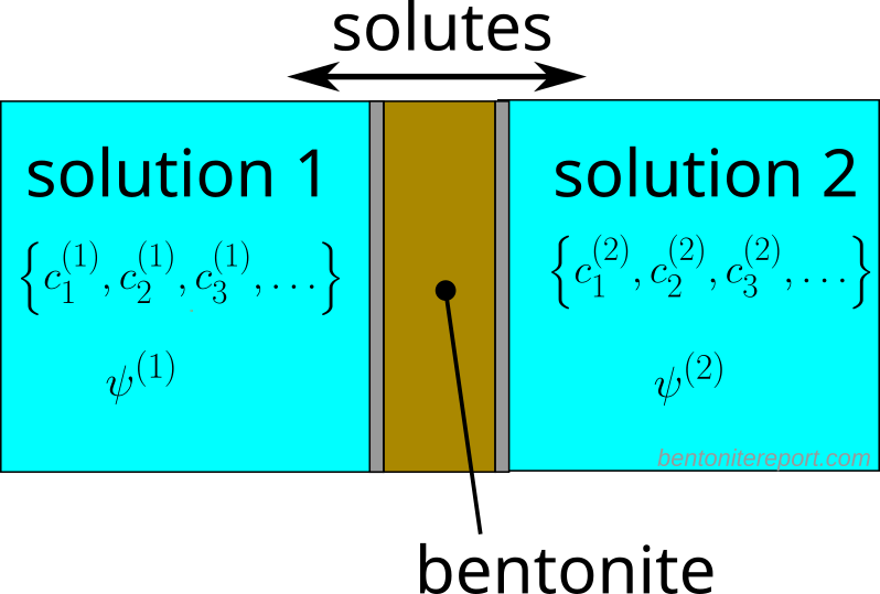
The external solutions (labeled “1” and “2”) are specified by general species compositions, with the only constraint that they should be electrically neutral. We consequently consider a situation with possible chemical gradients — and corresponding mass transfer — across the bentonite sample, while the hydrostatic pressures in the two reservoirs are assumed equal.3 The values of the electric potential in the external solutions have been labeled \(\psi^{(1)}\) and \(\psi^{(2)}\), respectively.
Treating the bentonite as a single homogeneous phase, the electric potential has discontinuities at the external solution/clay interfaces, due to Donnan equilibrium. In addition, the potential may vary within the bentonite, due to diffusion of charged species with different mobilities (electromigration). Schematically, the steady-state electric potential profile can be illustrated like this
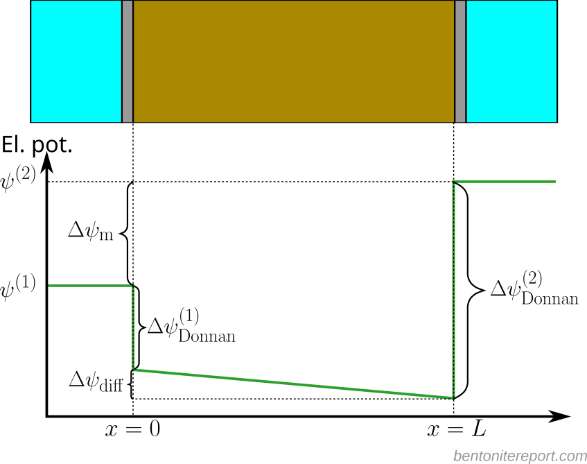
Here, \(\Delta \psi_\mathrm{Donnan}^{(1)}\) and \(\Delta \psi_\mathrm{Donnan}^{(2)}\) denote the potential changes due to Donnan equilibrium at the two interfaces.4 \(\Delta \psi_\mathrm{diff}\), which conventionally is named the diffusion potential, denotes the total change in potential across the sample due to electromigration. The membrane potential, \(\Delta \psi_\mathrm{m}\), can be expressed
\begin{equation} \Delta \psi_\mathrm{m} = \psi^{(2)} – \psi^{(1)} = \Delta \psi^{(1)}_\mathrm{Donnan} + \Delta \psi^{(2)}_\mathrm{Donnan} + \Delta \psi_\mathrm{diff} \tag{1} \end{equation}
Given the reservoir concentrations, the Donnan contributions can be calculated using the general framework, if also a value of \(c_\mathrm{IL}\) — which expresses the montmorillonite structural charge as a monovalent interlayer species concentration — is specified for the bentonite component. Such calculations also provide the corresponding sets of internal interface concentrations, i.e. \(\left \{c_{1}^\mathrm{int}(0), c_{3}^\mathrm{int}(0), c_{3}^\mathrm{int}(0), \ldots \right \}\), and \(\left \{c_{1}^\mathrm{int}(L), c_{3}^\mathrm{int}(L), c_{3}^\mathrm{int}(L), \ldots \right \}\), where we denote by \(c_i^\mathrm{int}(x)\) the concentration for species \(i\) at position \(x\) within the clay, and we assume the clay domain located between \(x=0\) and \(x=L\).
The sets of internal interface concentrations, in turn, constitute boundary conditions for solving e.g. the Nernst-Planck equation in the clay domain. Within the Nernst-Planck framework, the gradient of the electrostatic potential in the clay is expressed in terms of species concentrations and diffusivities as
\begin{equation} \nabla \psi(x) = – V_T \cdot \frac{\sum z_i\cdot D_i \cdot \nabla c_i^\mathrm{int} (x) }{\sum z_i^2\cdot D_i \cdot c_i^\mathrm{int} (x)} \tag{2} \end{equation}
where \(z_i\) and \(D_i\) denote, respectively, the charge number and diffusion coefficient in the clay domain, for species \(i\), and \(V_T = RT/F\) is the thermal voltage (we assume \(V_T\) = 25.7 mV here). From eq. 2 the diffusion potential can be evaluated.
Note that the problem of ending up with a too constrained model when both the Donnan equilibrium and the Nernst-Planck frameworks are invoked does not occur here. This is in contrast to the problems we recently discussed in the model of Tournassat and Steefel (2015). That model requires Donnan equilibrium at each point within the clay, while here it is only imposed at the two interface points.
In the following we will evaluate the membrane potential numerically in some different cases. We start, however, by analyzing the 1:1 system analytically, in order to get a better feel for these processes in compacted bentonite.
1:1 system
The pure 1:1 system has a single type of monovalent cation and a single type of monovalent anion (e.g. Na-montmorillonite in contact with NaCl solutions). The requirement of charge neutrality dictates equal concentrations of cations (\(c_+\)) and anions (\(c_-\)) in each external solution, and we write
\begin{equation} c_+^{(n)} = c_-^{(n)} = c^{(n)} \tag{3} \end{equation}
where \(c^{(n)}\) is the electrolyte concentration in reservoir \(n\) (\(n\) = 1 or 2).
In this analytical treatment, we assume the often relevant condition of having small external concentrations as compared with the concentration of structural charge in the clay, i.e.
\begin{equation} c^{(n)} \ll c_\mathrm{IL},\tag{4} \end{equation}
where the amount of structural charge is quantified by
\begin{equation} c_\mathrm{IL} = \frac {CEC\cdot\rho_w}{F\cdot w}. \tag{5} \end{equation}
Here \(CEC\) is the cation exchange capacity, \(w\) the water-to-solid mass ratio, \(\rho_w\) is water density and \(F\) the Faraday constant.
Under the condition expressed in eq. 4, the so-called Donnan factors (\(f_D\)) can be approximated as
\begin{equation} f_D^{(n)} \equiv e^{\psi^{\star, (n)}/V_T}\approx \tag{6} \frac{c^{(n)}}{c_\mathrm{IL}} \end{equation}
where \(\psi^{\star, (n)}\) is the Donnan potential. In eq. 6 we have ignored the activity coefficient correction factor; contributions to the membrane potentials from activity coefficient differences are expected to be small, and here we will not consider them.5 Note that Donnan potentials are negative, and that \(\Delta \psi_\mathrm{Donnan}^{(1)} = \psi^{\star, (1)}\) and \(\Delta \psi_\mathrm{Donnan}^{(2)} = -\psi^{\star, (2)}\). Utilizing eq. 6, we can express the total Donnan contribution to the membrane potential as6
\begin{equation} \Delta \psi_\mathrm{Donnan} = \Delta \psi^{(1)}_\mathrm{Donnan} + \Delta \psi^{(2)}_\mathrm{Donnan} \approx V_T\ln{\frac{c^{(1)}}{c^{(2)}}} \tag{7} \end{equation}
For the clay domain, the requirement of charge neutrality can be written
\begin{equation} c_+^\mathrm{int}(x) = c_\mathrm{IL}+c_-^\mathrm{int}(x) \tag{8} \end{equation}
from which it follows that the gradients of anion and cation concentrations are equal
\begin{equation} \nabla c_+^\mathrm{int}(x) = \nabla c_-^\mathrm{int}(x) \tag{9} \end{equation}
We can therefore approximate the gradient of the electric potential in the clay (eq. 2) as
\begin{equation} \nabla \psi(x) \approx V_T \frac{\left ( D_-/D_+-1 \right)}{c_\mathrm{IL} } \nabla c_-^\mathrm{int}(x) \tag{10} \end{equation}
where we also have continued assuming low external concentrations (eq. 4).
If we impose a constant internal concentration gradient, i.e. \(\nabla c_-^\mathrm{int} (x) = \Delta c_-^\mathrm{int}/L\), where \(\Delta c_-^\mathrm{int} \equiv c_-^\mathrm{int}(L) – c_-^\mathrm{int}(0)\), the diffusion potential can be written
\begin{equation} \Delta \psi_\mathrm{diff} \approx V_T \frac{\left ( D_-/D_+-1 \right )}{c_\mathrm{IL} } \Delta c^\mathrm{int}_-\tag{11} \end{equation}
Combining eqs. 7 and 11 gives an approximation for the membrane potential for a 1:1 system, valid for low external concentrations
\begin{equation} \psi_\mathrm{m} \approx \left ( \ln{\frac{c^{(1)}}{c^{(2)}}} + \frac {\left ( D_-/D_+-1 \right )}{c_\mathrm{IL} } \Delta c^\mathrm{int}_- \right ) V_T \tag{12} \end{equation}
The first term — the ideal Donnan contribution — depends only on the ratio of the concentration in the two reservoirs, and usually dominates over the diffusion potential (second term).
The diffusion potential is expected to be small under most circumstances, as it is seen to explicitly depend on \(1/c_\mathrm{IL}\). This behavior reflects that potential variations within the bentonite are reduced due to the presence of counter-ions (bentonite is a decent conductor). But the factor \(\Delta c_-^\mathrm{int}\) in eq. 11 contributes with an additional factor \(1/c_\mathrm{IL}\) to the diffusion potential, because of Donnan equilibrium (see eq. 6)
\begin{equation} \Delta c_-^\mathrm{int} = f_D^{(2)}c^{(2)} – f_D^{(1)}c^{(1)} \approx \frac {\left ( c^{(2)} \right )^2 – \left ( c^{(1)} \right )^2} {c_\mathrm{IL}} \tag{13} \end{equation}
Note also that the diffusion potential only depends on the relative values of the diffusivities, and consequently vanishes if there is no difference in mobility between the cation and the anion.
Comparisons with experiment
We can compare the present theory and approximations with measurements reported in Yaroshchuck et al. (2007). In this study, the membrane potential (called the “concentration potential”) was measured across sodium montmorillonite of density 2.0 g/cm3, with one external solution kept at 0.1 M NaCl and the other raised to 0.2 M, 0.3 M, or 0.5 M. The very high density corresponds to a value of \(c_\mathrm{IL} \approx\) 6.0 M,7 and thus eq. 12 applies (see eq. 4).
In order to also investigate the influence of a diffusion potential we should adopt values for the individual diffusivities of chloride and sodium. Experimental tracer diffusion results indicate that these ions have quite similar mobility. E.g., in pure Na-montmorillonite at 1.8 g/cm3 and 298 K, Kozaki et al. (1999, 2001, 2005) report values in the range \(1.5\cdot 10^{-11}\) — \(2.5\cdot 10^{-11}\) m2/s for chloride, and \(2.1\cdot 10^{-11}\) — \(2.4\cdot 10^{-11}\) m2/s for sodium. From these values we can estimate a range for the factor (\(D_-/D_+-1\)) of -0.4 — 0.2. Rather than adopting such a value, however, we here assume the diffusivities to have the corresponding bulk water ratio (1.53), giving \((D_-/D_+ -1)\) = 0.53. This is similar to the treatment in the examples in Tournassat and Steefel (2015), which we have discussed recently. Theoretical and experimental results are compared in the table below
Evaluations using cIL = 6.0 M, c(2) = 0.1 M, (D–/D+ – 1) = 0.53:
| App- | rox- | ima- | tion | Full | Frame- | work | Exp. | ||||
| \(c^{(1)}\) (M) | \(\psi^{\star,(1)}\) (mV) | \(\psi^{\star,(2)}\) (mV) | \(\Delta \psi_\mathrm{D}\) (mV) | \(\Delta\psi_\mathrm{diff}\) (mV) | \(\psi_\mathrm{m}\) (mV) | \(\psi^{\star,(1)}\) (mV) | \(\psi^{\star,(2)}\) (mV) | \(\Delta \psi_\mathrm{D}\) (mV) | \(\Delta\psi_\mathrm{diff}\) (mV) | \(\psi_\mathrm{m}\) (mV) | \(\psi_\mathrm{m}\) (mV) |
| 0.2 | -87.4 | -105.2 | 17.8 | -0.011 | 17.8 | -87.4 | -105.2 | 17.8 | -0.011 | 17.8 | 18 |
| 0.3 | -77.0 | -105.2 | 28.2 | -0.030 | 28.2 | -77.1 | -105.2 | 28.1 | -0.030 | 28.1 | 28 |
| 0.5 | -63.9 | -105.2 | 41.4 | -0.090 | 41.3 | -64.0 | -105.2 | 41.2 | -0.088 | 41.1 | 41 |
This table compares calculations performed using eq. 12 (columns 2 — 6), calculations performed using the full frameworks for Donnan equilibrium and the Nernst-Planck potential (columns 7 — 11), and experimental values (last column). We note that, for this very high value of \(c_\mathrm{IL}\), the calculated Donnan contributions (\(\Delta \psi_\mathrm{D}\)) are essentially identical whether or not the full framework is adopted. We also see that the calculated diffusion potential contributions are completely negligible: the largest value calculated is still below 0.1 mV! Finally, we note excellent agreement between calculated and measured membrane potentials.
The agreement with experiment suggests, not only that the membrane potential is completely determined by Donnan equilibrium in these systems, but that bentonite essentially play by the same rules as conventional ion-exchange membranes.2 In particular, these results8 are even more evidence for that all exchangeable cations are mobile in bentonite.
To explore the NaCl system further, let’s investigate how the results change for lower clay density. In the tables below are shown corresponding results as above, but for \(c_\mathrm{IL}\) = 3.0 M and \(c_\mathrm{IL}\) = 1.5 M, which roughly correspond to densities 1.6 g/cm3 and 1.1 g/cm3, respectively.
Evaluations using cIL = 3.0 M, c(2) = 0.1 M, (D–/D+ – 1) = 0.53:
| App- | rox- | ima- | tion | Full | Frame- | work | ||||
| \(c^{(1)}\) (M) | \(\psi^{\star,(1)}\) (mV) | \(\psi^{\star,(2)}\) (mV) | \(\Delta \psi_\mathrm{D}\) (mV) | \(\Delta\psi_\mathrm{diff}\) (mV) | \(\psi_\mathrm{m}\) (mV) | \(\psi^{\star,(1)}\) (mV) | \(\psi^{\star,(2)}\) (mV) | \(\Delta \psi_\mathrm{D}\) (mV) | \(\Delta\psi_\mathrm{diff}\) (mV) | \(\psi_\mathrm{m}\) (mV) |
| 0.2 | -69.6 | -87.4 | 17.8 | -0.045 | 17.8 | -69.7 | -87.4 | 17.7 | -0.044 | 17.7 |
| 0.3 | -59.2 | -87.4 | 28.2 | -0.120 | 28.1 | -59.4 | -87.4 | 28.0 | -0.116 | 27.9 |
| 0.5 | -46.0 | -87.4 | 41.4 | -0.361 | 41.0 | -46.7 | -87.4 | 40.7 | -0.336 | 40.4 |
Evaluations using cIL = 1.5 M, c(2) = 0.1 M, (D–/D+ – 1) = 0.53:
| App- | rox- | ima- | tion | Full | Frame- | work | ||||
| \(c^{(1)}\) (M) | \(\psi^{\star,(1)}\) (mV) | \(\psi^{\star,(2)}\) (mV) | \(\Delta \psi_\mathrm{D}\) (mV) | \(\Delta\psi_\mathrm{diff}\) (mV) | \(\psi_\mathrm{m}\) (mV) | \(\psi^{\star,(1)}\) (mV) | \(\psi^{\star,(2)}\) (mV) | \(\Delta \psi_\mathrm{D}\) (mV) | \(\Delta\psi_\mathrm{diff}\) (mV) | \(\psi_\mathrm{m}\) (mV) |
| 0.2 | -51.8 | -69.6 | 17.8 | -0.18 | 17.6 | -52.2 | -69.7 | 17.5 | -0.170 | 17.3 |
| 0.3 | -41.4 | -69.6 | 28.2 | -0.48 | 27.8 | -42.3 | -69.7 | 27.4 | -0.434 | 26.9 |
| 0.5 | -28.2 | -69.6 | 41.4 | -1.44 | 39.9 | -30.7 | -69.7 | 39.0 | -1.146 | 37.8 |
For \(c_\mathrm{IL}\) = 3.0 M, the difference between using the full framework or eq. 12 is seen to still only affect the evaluated membrane potentials on the order of tenths of mV. Only for the higher external concentrations in the system with \(c_\mathrm{IL}\) = 1.5 M are the differences becoming above 1 mV. Similarly, the diffusion potential is seen to be essentially negligible for all these cases.
Further investigation of potentials and fluxes
It should be emphasized that we are not actually solving the full Nernst-Planck transport framework in these examples. Rather, we calculate the corresponding potential difference as we impose a linear internal concentration profile. This is similar to the evaluation made by Tournassat and Steefel (2015) — although they impose concentration profiles in a presumed bulk water phase within the clay. Similar to that publication, we will here visualize the corresponding fluxes in some cases of interest.
The total flux of a charged species in the Nernst-Planck framework can be written as the sum of a “Fickian” contribution (i.e. proportional to the corresponding concentration gradient) and a contribution from electromigration (i.e. flux induced by the presence of an electric field).9
\begin{equation} j_\mathrm{tot} = j_\mathrm{conc} + j_\mathrm{E} \tag{14} \end{equation}
where the “Fickian” flux is given by
\begin{equation} j_\mathrm{conc} = -D\cdot\nabla c^\mathrm{int}(x) \tag{15} \end{equation}
and the electromigration term is given by
\begin{equation} j_\mathrm{E} = -z\cdot D\cdot c^\mathrm{int}(x)\frac{\nabla \psi(x)}{V_T} \tag{16} \end{equation}
NaCl
Below are plotted imposed concentration profiles, Nernst-Planck fluxes, and the electric potential profile, for the NaCl-system with \(c_\mathrm{IL}\)=3.0 M, \(c^{(1)}\) = 0.5 M, and \(c^{(2)}\) = 0.1 M (for which we previously calculated \(\Delta \psi_\mathrm{m}\) = 40.4 mV and \(\Delta \psi_\mathrm{diff}\) = -0.3 mV). To calculate fluxes we must choose absolute values of the diffusion coefficients, which we take to be \(D_\mathrm{Na}=1.33\cdot 10^{-10}\) m2/s and \(D_\mathrm{Cl}=2.03\cdot 10^{-10}\) m2/s.10
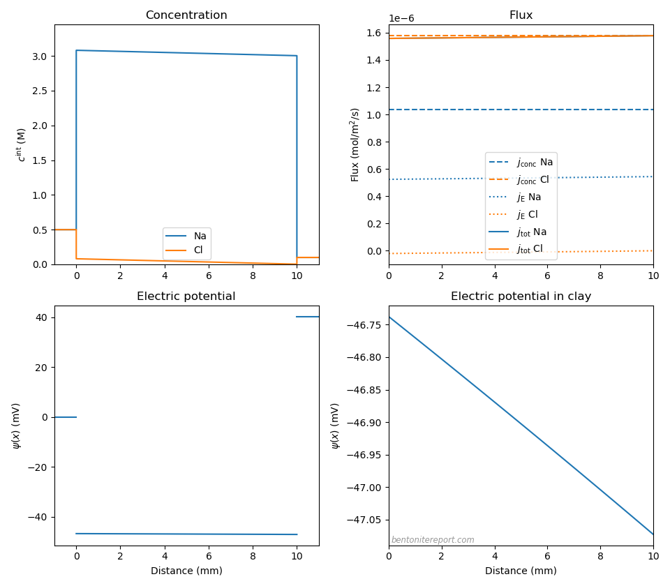
The total NaCl flux is essentially constant throughout the sample (we have adopted a sample length of 10 mm), demonstrating that the imposed linear concentration profile in essence is the steady-state solution. We see that the flux of chloride — which has a much smaller concentration than sodium — is completely dominated by the concentration gradient contribution (eq. 15), while the sodium flux has significant contributions from both the concentration gradient and the electric field (eq. 16). The picture is clear: the faster chloride ions diffuse with a rate set by their individual diffusion coefficient, while the induced electric field boosts the less mobile (but more abundant) sodium ions in order to “keep up”. The behavior is similar to what would be experienced in a bulk solution with a NaCl gradient. In that case, however, the chloride is as much retarded as the sodium is boosted, resulting in a diffusivity for the full salt that is between the two individual values. In compacted bentonite, on the other hand, the electromigration flux is mainly significant for sodium (the counter-ions). Therefore the full salt diffuse with a rate essentially set by the chloride mobility.
We can quantify the relative influcence of electromigration for a specific species by taking the ratio of eqs. 15 and 16, and also utilizing the approximation for \(\nabla \psi (x)\) in eq. 10
\begin{equation} \frac{j_\mathrm{E}}{j_\mathrm{conc}} \approx \frac{z\cdot c^\mathrm{int}(x)} {c_\mathrm{IL}} \left (D_\mathrm{Cl}/D_\mathrm{Na}- 1 \right ) \tag{17} \end{equation}
This expression explicitly shows that the electromigration flux is negligible for chloride (because \(c^\mathrm{int}_\mathrm{Cl}(x) \ll c_\mathrm{IL}\)), while the \(j_\mathrm{E}/j_\mathrm{conc}\)-ratio for sodium is essentially determined by the factor \(\left (D_\mathrm{Cl}/D_\mathrm{Na} – 1 \right )\) (because \(c^\mathrm{int}_\mathrm{Na}(x) \approx c_\mathrm{IL}\)).
For a similar NaCl-system at lower density, the picture is quite similar (here \(c_\mathrm{IL}\)=1.5 M, with the other parameters as previously; \(\Delta \psi_\mathrm{m}\) = 37.8 mV and \(\Delta \psi_\mathrm{diff}\) = -1.1 mV)

Let’s also play with the relative mobility between anion and cation. In the plot below we have decreased the chloride diffusivity to \(D_\mathrm{Cl}=0.133\cdot 10^{-10}\) m2/s, while keeping with the same values as before for the other parameters (for \(c_\mathrm{IL}\) = 3.0 M).

In this case, the diffusivity factor for the electromigration is \((D_-/D_+ -1) = -0.9\). The negative value indicates an electric field directed in the opposite direction as compared to the previous cases (chloride is now the slower ion). The diffusion potential is \(\Delta \psi_\mathrm{diff}\) = +0.6 mV, which still is quite small, given that the chloride is assumed to have ten times lower mobility as compared with sodium. The evaluated membrane potential is \(\Delta \psi_\mathrm{m}\) = 41.3 mV. We note that the flux is constant throughout the domain and that chloride is completely governed by the concentration gradient contribution, while the sodium flux is composed of two oppositely directed much larger contributions of similar magnitude.
If we instead make the sodium diffusivity 10 times smaller than the chloride diffusivity (\(D_\mathrm{Na}=0.203\cdot 10^{-10}\) m2/s, \(D_\mathrm{Cl}=2.033\cdot 10^{-10}\) m2/s), the effect is more dramatic
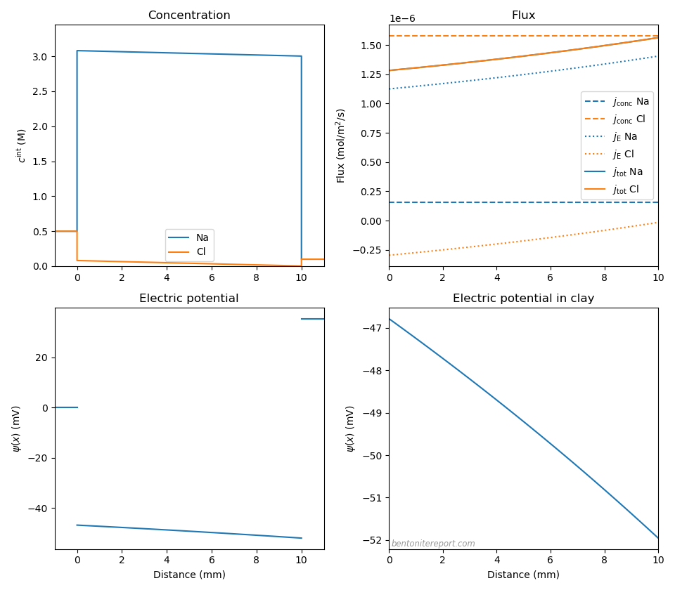
With \((D_-/D_+ -1)\) = 9.0, the diffusion potential becomes considerably larger than in any of our previously investigated cases: \(\Delta \psi_\mathrm{diff}\) = -5.2 mV (\(\Delta \psi_\mathrm{m}\) = 35.5 mV). This is reasonable, since a significantly smaller mobility of the counter-ions requires a larger electric field to produce similar fluxes. The sodium flux is therefore dominated by electromigration, and we also note a non-negligible contribution from electromigration for chloride. The overall flux varies quite significantly throughout the clay domain; we’re not really in steady-state.
“Uphill” diffusion
With a solid understanding of the principles for diffusion of a 1:1 electrolyte in compacted bentonite, let’s turn our attention to the “uphill” test (Glaus et al., 2013). The conditions for the main electrolyte (NaClO4) and clay in this study are the same as in our previous case: one reservoir is at concentration 0.1 M, and one at 0.5 M, and the clay is pure high-density Na-montmorillonite. For a further discussion of this study, see this previous post. Here we adopt the value \(c_\mathrm{IL}\) = 4.5 M and set \(c^{(1)}\) = 0.1 M and \(c^{(2)}\) = 0.5 M (in order to have a positive tracer flux). In addition to a main electrolyte, the “uphill” test has a sodium tracer (\(^{22}\mathrm{Na}\)) as a third component, with equal concentration in the two reservoirs (\(10^{-11}\) M). Here we choose sodium diffusivity \(D_\mathrm{Na}=3\cdot 10^{-11}\) m2/s, similar to what is evaluated in Glaus et al. (2007) and Birgersson and Karnland (2009). For perchlorate we choose \(D_\mathrm{ClO_4}=4\cdot 10^{-11}\) m2/s, in order to keep the same diffusivity ratio as for bulk (the perchlorate bulk value is \(1.79\cdot 10^{-9}\) m2/s (Heil, 1995)).
Since the only difference between the “uphill” study and the pure 1:1 case is the presence of a tracer, it is no surprise that concentrations, fluxes and potential behave very similarly
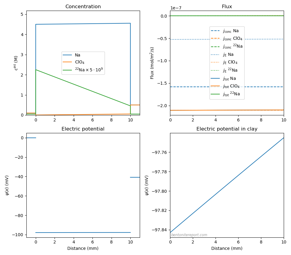
The membrane potential is here \(\Delta \psi_\mathrm{m} = -41.0\) mV, which is essentially identical to what we have evaluated for the NaCl system (the minus sign simply reflects that the left reservoir here has the lower concentration). With a smaller mobility difference between anion and cation, the diffusion potential is even more negligible than for NaCl, \(\Delta \psi_\mathrm{diff} = 0.1\) mV. The tracer flux is not resolved in the above plot, but looks like this
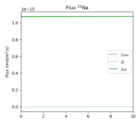
An analytical evaluation of the \(j_\mathrm{E}/J_\mathrm{conc}\)-ratio becomes a bit more complicated for the tracer as compared with the main salt (eq. 17). At the two interfaces, it can be shown that11
\begin{equation} \frac{j_\mathrm{E,^{22}Na}}{j_\mathrm{conc,^{22}Na}} \approx -\frac{c^\mathrm{(2)} \left ( c^{(1)} + c^{(2)} \right )} {c_\mathrm{IL}^2} \left (D_\mathrm{ClO_4}/D_ \mathrm{Na}- 1 \right ),\;\;\;\; x=0 \tag{18} \end{equation}
and
\begin{equation} \frac{j_\mathrm{E,^{22}Na}}{j_\mathrm{conc,^{22}Na}} \approx -\frac{c^\mathrm{(1)} \left ( c^{(1)} + c^{(2)} \right )} {c_\mathrm{IL}^2} \left (D_\mathrm{ClO_4}/D_ \mathrm{Na}- 1 \right ),\;\;\;\; x=L \tag{19} \end{equation}
We see that this ratio is expected to be small as long as the reservoir concentrations are small as compared with \(c_\mathrm{IL}\). This is also confirmed in the above plot; the electromigration contribution is completely negligible.
This result is the ultimate support for the claim I made in the “uphill” blog post: the phenomena is first and foremost an effect of ordinary Donnan equilibrium, just as conventional cation tracer diffusion is explained. Here we have explicitly included the electric potential in the analysis, and not only showed that electromigration is negligible for the tracer component, but qualitatively described how and where possible effects due to ion mobility differences occur in the set-up as a whole.
Tertre et al. (2024) — the publication critisized in the “uphill” blog post — states that the “uphill” study
[…] demonstrated the marked influence of background electrolyte concentration gradient on tracer diffusion, and thus the necessity to understand the couplings between diffusion of several charged species present at contrasting concentrations and experiencing different concentration gradients.
In contrast to Tertre et al. (2024), we have here presented this understanding and — in contrast to the statement — demonstrated that the “uphill” effect does not depend critically on any additional mechanisms or couplings as compared with conventional cation tracer diffusion.
As for the previous cases, we can play around with the parameters to explore more “extreme” conditions in an “uphill” test. Here we have increased the perchlorate diffusivity to \(D_\mathrm{ClO_4}=9\cdot 10^{-11}\) m2/s (i.e. three times the sodium diffusivity), and lowered \(c_\mathrm{IL}\) to \(c_\mathrm{IL} = \) 2.0 M (corresponding roughly to a density of 1.25 g/cm3).
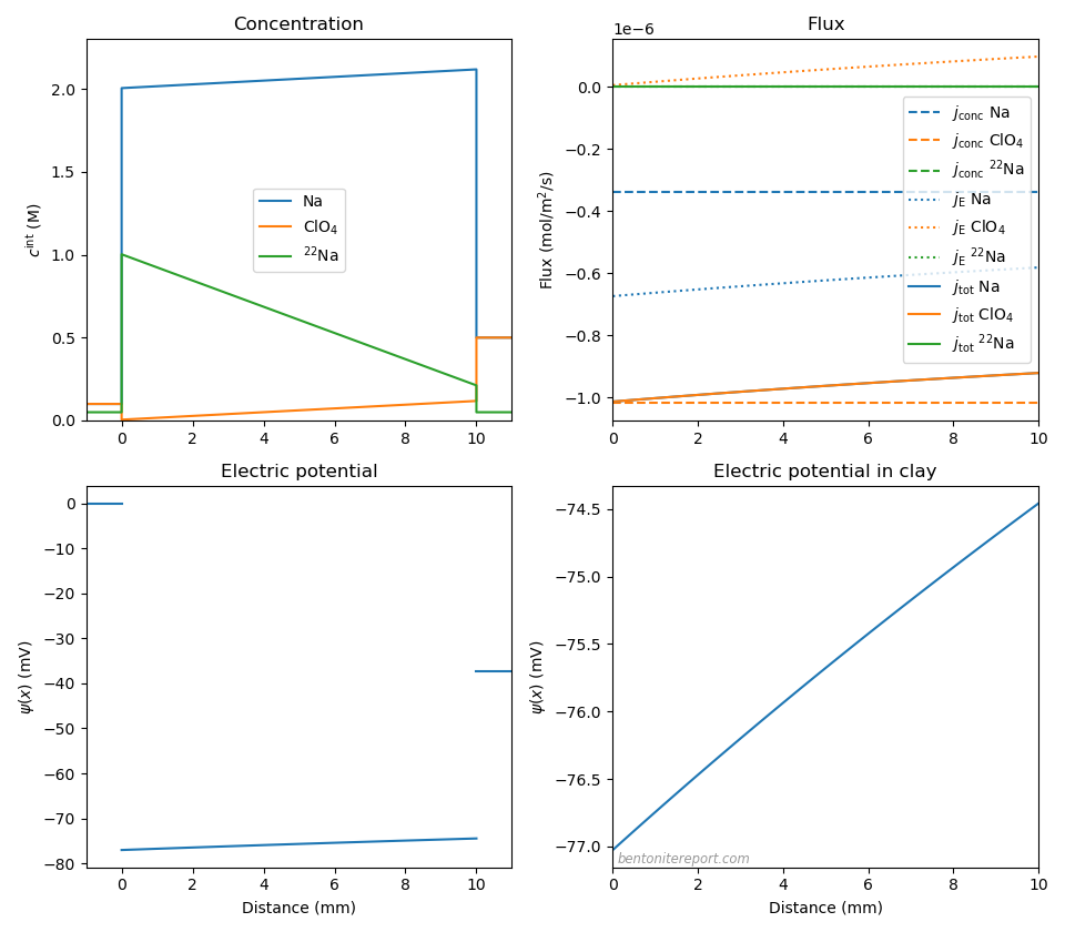
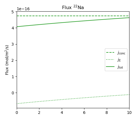
Predictably, the main counter-ion transport is now dominated by electromigration, and we see some influence of electromigration also on the perchlorate and the sodium tracer. Nevertheless, even for this extreme case, the “uphill” tracer flux is mainly “Fickian” and is principally explaind as an effect due to Donnan equilibrium at the sample interfaces. For this case we have \(\Delta \psi_\mathrm{m}\) = -37.4 mV and \(\Delta \psi_\mathrm{diff}\) = 2.6 mV.
Update (261006): The “uphill” test is modeled with the full Nernst-Planck framework here.
CaCl2
Let’s also examine the pure 2:1 system, which corresponds e.g. to CaCl2 solutions in contact with Ca-montmorillonite. As we discussed in a recent blog post, the Donnan equilibrium for this system is quite different as compared with the 1:1 system. This will naturally also impact the membrane potential. Moreover, experiments indicate that calcium diffuses several times slower than chloride in bentonite (Kozaki et al., 2000), which suggests a larger effect on the diffusion potential. But, similar to previous cases, let’s begin by assuming the same diffusivity ratio as for bulk. With \(D_\mathrm{Cl}=2.03\cdot 10^{-10}\) m2/s, \(D_\mathrm{Ca}=0.79\cdot 10^{-10}\) m2/s, \(c_\mathrm{IL} = \) 3.0 M, and having \(c^{(1)}\) = 0.25 M and \(c^{(2)}\) = 0.05 M12 we get the following picture
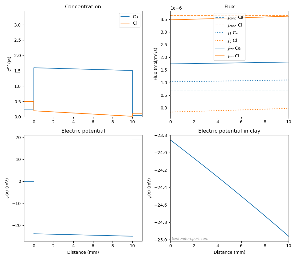
The membrane potential is here \(\Delta \psi_\mathrm{m} = 18.8\) mV and the diffusion potential \(\Delta \psi_\mathrm{diff} = -1.1\) mV. Thus, even if the relative influence of the diffusion potential is larger han for NaCl, the main contribution to the membrane potential is still due do Donnan equilibrium; the considerably lower membrane potential in this case (about half of the NaCl value with the same amount of chloride in the reservoirs) is primarily a consequence of Donnan equilibrium: the Donnan factors have in this case a square-root dependence on external concentration. However, as a consequence of calcium mobility being considerably lower than sodium mobility (\(D_-/D_+ – 1\) = 1.57), the magnitude of the diffusion potential is about three times larger than for the NaCl case. The resulting flux is also seen to be not completely constant throughout the clay domain. Nevertheless, the same qualitative picture of the transport mechanism as for NaCl is valid here: chloride transport is dominated by its “Fickian” contribution, diffusing with the rate set by the individual mobility, while the less mobile calcium is boosted by an electromigration contribution, which here is actually larger than its concentration gradient contribution. The salt as a whole diffuses with the rate essentially set by the chloride diffusivity.
Let’s also explore an “extreme” case. Below we have set the Ca mobility to be a factor 10 lower than Cl (\(D_\mathrm{Cl}=2.03\cdot 10^{-10}\) m2/s, \(D_\mathrm{Ca}=0.203\cdot 10^{-10}\) m2/s) and lowered \(c_\mathrm{IL}\) to \(c_\mathrm{IL} = \) 1.5 M.
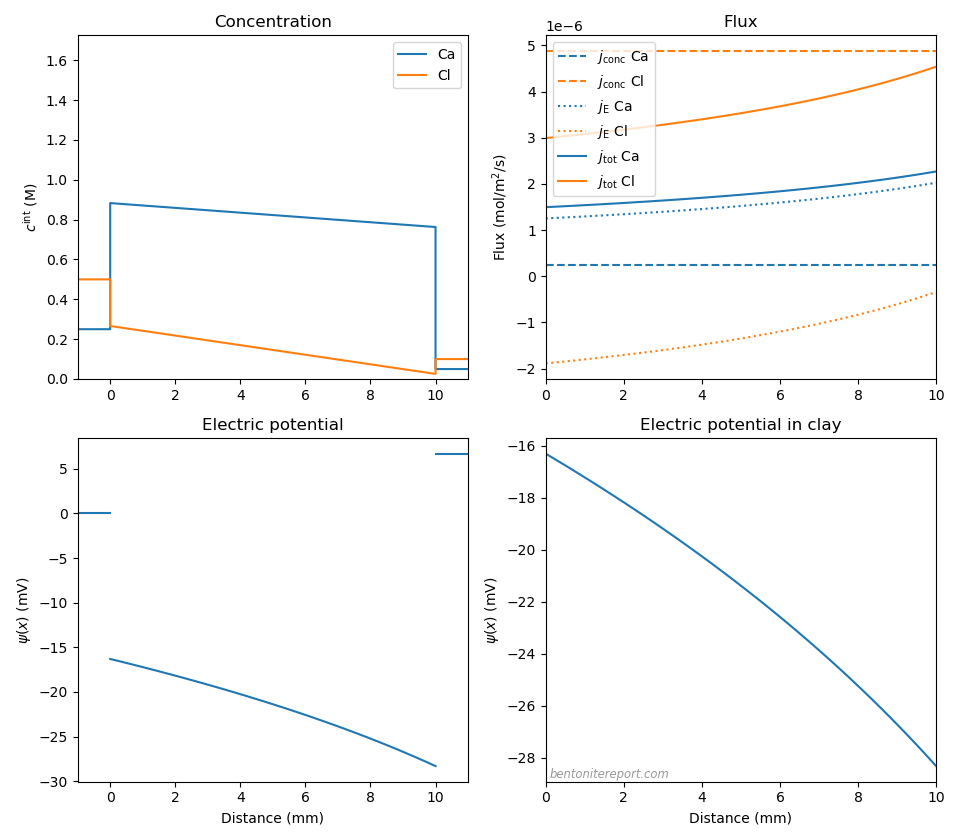
Here the membrane potential is only \(\psi_\mathrm{m} = 6.7\) mV due to a large contribution from the diffusion potential (\(\Delta \psi_\mathrm{diff} = -12.0\) mV), The calcium flux is seen to be strongly dominated by electromigration, and chloride transport is also strongly affected. We are far from steady-state.
Mixing sodium and calcium
As a final case we consider systems containing both a mono- and a di-valent type of cation. Since cation concentrations are enhanced within the clay, a significant diffusion potential may develop, even for relatively small variations of the external solutions. For instance, with a pure 0.1 M NaCl solution on one side (2), and a mixture of 0.003 M CaCl2 and 0.094 M NaCl on the other (1), we get the following result
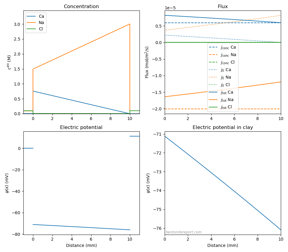
Here we have assumed \(c_\mathrm{IL} = \) 3.0 M, \(D_\mathrm{Cl}=2.03\cdot 10^{-10}\) m2/s, \(D_\mathrm{Ca}=0.79\cdot 10^{-10}\) m2/s, and \(D_\mathrm{Na}=1.33\cdot 10^{-10}\) m2/s.
Note that the Donnan equilibrium at the left interface acts as to make the clay contain 50% sodium and 50% calcium (charge wise) even though the calcium content in the reservoir is only 6%! A quite minor “disturbance” in the external solution consequently induce huge transport processes.13 This transport is essentially independent of the presence of an anion, and is governed by mutual diffusion of calcium and sodium. The mobility difference for these two ions thus results in a large diffusion potential: \(\Delta \psi_\mathrm{diff}\) = -5.0 mV. The membrane potential is quite substantial: \(\Delta \psi_\mathrm{m}\) = 11.4 mV. The calcium transport is dominated by the concentration gradient flux, while the oppositely directed sodium flux is more profoundly retarded by the electric field (although it is still dominated by the concentration gradient). We conclude that the full Na-Ca transport process occurs approximately at the rate set by the individual mobility for calcium. This process is essentially charge neutral, i.e. as much Ca charge is transported to the right as Na charge is transported to the left.
It may also be worth noticing that although the chloride concentration is the same in the two external solutions, an internal gradient — and a corresponding chloride flux — is induced
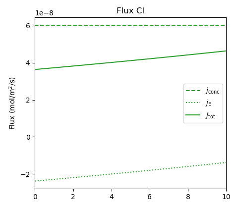
This chloride flux, which is directed to the right and seen to be quite influenced (retarded) by electromigration, is more than two orders of magnitude smaller than the Ca-Na flux. This result implies that also anions may experience seeming “uphill” diffusion (though I’m not sure how easy it would be to detect experimentally).
A lesson here is that calcium concentrations often must be very small in order to be treated as a tracer when added to a sodium system. For example, Tinnacher et al. (2016) incorrectly treats calcium as a tracer when adding 0.001 M CaBr2 to an otherwise pure 0.1 M NaCl-montmorillonite system at 0.8 g/cm3.14 At that density, we may approximate \(c_\mathrm{IL} = 1.0\) M, which gives the following situation (\(D_\mathrm{Cl} = 2.03 \cdot 10^{-10}\) m2/s, \(D_\mathrm{Br}=2.01\cdot 10^{-10}\) m2/s, \(D_\mathrm{Ca}=0.79\cdot 10^{-10}\) m2/s, and \(D_\mathrm{Na}=1.33\cdot 10^{-10}\) m2/s; CaBr2 in reservoir 1)
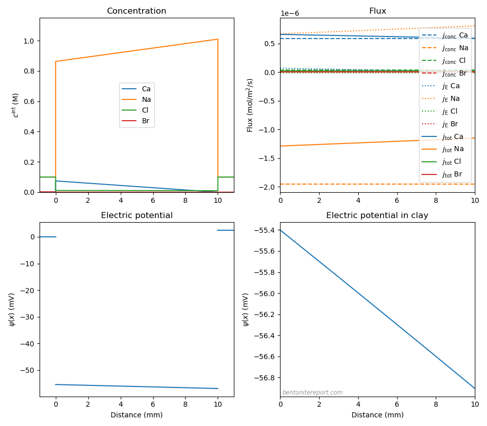
The amount of calcium in the clay at the left interface is in this case predicted to be about 15% — which certainly cannot be regarded a trace level. Consequently, the main mode of transport in this test is oppositely directed sodium and calcium fluxes that essentially does not involve the anions. In addition, we predict a non-zero membrane potential of \(\Delta \psi_\mathrm{m} = 2.5\) mV, with \(\Delta \psi_\mathrm{diff} = -1.5\) mV.
The bromide, in contrast, can be treated as tracer, and its flux look like this

This flux is about two orders of magnitude smaller than the dominating Ca-Na flux,15 and is seen to be essentially unaffected by the electric field (i.e. mainly “Fickian”).
Additional comments
Here we have investigated transport processes that occur in the presence of chemical gradients between two external reservoirs sandwiching a compacted bentonite component. For this case, compacted bentonite appears to function similar to a conventional charged ion exchange membrane.2 However, compacted bentonite used e.g. for waste storage is quite different from ordinary ion exchange membranes, in that we are more interested in what is going on inside it, rather than directly utilizing its semi-permeable properties. The results discussed in this blog post are useful when interpreting tests that involve bentonite sandwiched between external solutions. For a description of what is going on inside the bentonite component, such results and tests may be very useful, but do not provide a full picture.
As with many topics discussed on the blog, I find the lack of relevant experimental results quite extraordinary. I mean that many labs should routinely measure membrane potentials as part of exploring bentonite systems. Instead, as far as I understand, the study by Yaroschchuck et al. (2007) is the only one published on actual compacted bentonite.16 Moreover, this study appears to be completely forgotten!8
Yaroschchuck et al. (2007) use extremely high density, and it would be interesting with data also at lower densities (1.6 — 1.3 g/cm3, say); the present theory predicts only minor changes in membrane potentials. A “simple” further test of the present description would be to measure the membrane potential in e.g. a pure CaCl2-montmorillonite system. We end this post by presenting such potentials as predicted from the present theory (the calculation uses \(D_\mathrm{Cl} = 2\cdot 10^{-10}\) m2/s and \(D_\mathrm{Ca} = 0.5\cdot 10^{-10}\) m2/s).
| \(c^{(1)}_\mathrm{Cl}\) | \(c^{(2)}_\mathrm{Cl}\) | \(\psi_m\) \(c_\mathrm{IL}\) = 6.0 M | \(\psi_m\) \(c_\mathrm{IL}\) = 2.0 M |
| 0.2 M | 0.1 M | 8.7 mV | 7.9 mV |
| 0.3 M | 0.1 M | 13.7 mV | 12.0 mV |
| 0.5 M | 0.1 M | 19.6 mV | 15.9 mV |
Update (260922): The full Nernst-Planck framework is treated within the homogeneous mixture model here.
Footnotes
[1] The focus here is on what I call simple ions, i.e. ions that only interact with the bentonite by beeing part of a diffuse layer. In bentonite, more complex processes are active for certain species that interact with e.g. montmorillonite edges. Here is presented an extension of the homogeneous mixture model for “truly” sorbing species.
[2] What is presented in this blog post is, as far as I understand, the “Teorell- Meyer-Sievers” model for the membrane potential, applied to compacted bentonite. This model, which was originally developed in the 1930s, is used routinely within the ion-exchange membrane scientific discipline. I’m currently reading up on this literature, and is here using my “usual” terminology (for bentonite). I have not yet come across sources with specific focus on bentonite/montmorillonite, and I’m not sure how well established these are as a membrane materials within this discipline. In a well-cited review by Xu (2005), bentonite is mentioned once — misspelled! Perhaps this is indicative of a missing link between the ion exchange membrane and compacted bentonite research fields.
[3] Although different water chemistries will induce different swelling pressure repsonses, and thus couple to mechanical processes in the bentonite, we here ignore pressure altogether (but we certainly will have reason to return to this).
[4] Note that Donnan potentials generally are negative, while \(\Delta \psi_\mathrm{Donnan}^{(1)}\) and \(\Delta \psi_\mathrm{Donnan}^{(2)}\) are negative or positive, depending on whether the contribution decreases or increases the potential as we move to the right.
[5] Including activity coefficients, eq. 6 becomes
\begin{equation} f_D^{(n)} \approx \gamma^{\mathrm{ext},(n)}/\gamma^\mathrm{int}\cdot c^\mathrm{(n)}/c_\mathrm{IL} \end{equation}
The expression for the membrane potential will contain the ratio of the Donnan factors at each interface
\begin{equation} V_T\ln(f_D^{(1)}/f_D^{(2)}), \end{equation}
and the interlayer activity coefficients (\( \gamma^\mathrm{int}\)) will therefore cancel (to the extent that the this quantity can be considered independent of external solution concentration). The contribution from Donnan equilibrium to the membrane potential thus become
\begin{equation} \Delta \psi_\mathrm{Donnan} \approx V_T(\ln{\frac {c^{(1)}}{c^{(2)}}} + \ln{\frac {\gamma^{\mathrm{ext},(1)}}{\gamma^{\mathrm{ext},(2)}}}). \end{equation}
The primary approximation made in the present treatment is to ignore the second term.
[6] This equation is often referred to as the Nernst equation. Note, however, that this quantity fundamentally involves two semi-permeable components. I have previously referred to a similar relation for a single interface as the Nernst equation.
[7] The value of \(c_\mathrm{IL}\) (eq. 5) depends on the cation exchange capacity of the material: montmorillonite “from Milos”. Different sources report this value in the range 0.80 — 0.85 eq./kg.
[8] The obscurity of Yaroshchuck et al. (2007) amazes me. This paper is part of a “trilogy” published in 2007, by the same authors (to a large extent). The other two studies are featured massively on the blog: Glaus et al. (2007) demonstrates that interlayer diffusion dominates mass transfer in compacted bentonite (see here and here), and Van Loon et al. (2007) is the only study that passed our assessment of published chloride equilibrium concentrations in compacted bentonite (see here, here, and here). Glaus et al. (2007) has at the moment 178 citations on Google Scholar, and Van Loon et al. (2007) has 333 citations. Yaroshchuck et al. (2007), in contrast, has 7 citations… Perhaps even more weirdly, Yaroshchuck et al. (2007) is not cited in Van Loon et al. (2007), although the former study presents the framework for Donnan equilibrium between compacted bentonite and a 1:1 electrolyte, and relates it to the findings of Glaus et al. (2007). It should thus had been an “easy win” for Van Loon et al. (2007) to provide a proper explanation for anion exclusion in bentonite, and to make the correct connection between anion and cation tracer through-diffusion. Instead, and for reasons I can’t get my head around, van Loon et al. (2007) get lost in ideas on “anion-accessible porosity”.
[9] Generally, the flux may also have an advective component, which we don’t consider here.
[10] The absolute values of the diffusivities are chosen rather arbitrarily; in this example we have adopted values ten times smaller than the corresponding values in bulk. The absolute value of the corresponding flux is therefore also arbitrary. Here, however, we are mainly interested in how constant the flux is throughout the clay, and in the relative contributions from concentrations and electric fields, rather than the absolute values. In some cases in this section we have adopted empirical values for diffusivities in order to compare also the absolute value of the flux.
[11] The electromigration and concentration gradient fluxes for the tracer in the “uphill” test can be written (see eqs. 15 and 16)
\begin{equation} j_\mathrm{E,tr} \approx -D_\mathrm{Na} \cdot c_\mathrm{tr}^\mathrm{int}(x) \cdot \left (D_\mathrm{ClO_4}/D_ \mathrm{Na}- 1 \right) \frac{\nabla c^\mathrm{int}_\mathrm{ClO_4}}{c_\mathrm{IL}} \end{equation}
\begin{equation} j_\mathrm{conc,tr} = -D_\mathrm{Na} \cdot \nabla c_\mathrm{tr}^\mathrm{int}(x) \end{equation}
Their ratio is
\begin{equation} \frac{j_\mathrm{E,tr}}{j_\mathrm{conc,tr}} \approx \frac{c_\mathrm{tr}^\mathrm{int}(x)}{c_\mathrm{IL}} \cdot \left (D_\mathrm{ClO_4}/D_ \mathrm{Na}- 1 \right) \cdot \frac{c^\mathrm{int}_\mathrm{ClO_4}(L) – c^\mathrm{int}_\mathrm{ClO_4} (0)}{c_\mathrm{tr}^\mathrm{int}(L) – c_\mathrm{tr}^\mathrm{int}(0)} \end{equation}
where we have explicitly written the gradients in terms of the internal interface concentrations. Using the relation between Donnan factors and concentrations, this concentration difference ratio can in turn be rewritten
\begin{equation} \frac{c^\mathrm{int}_\mathrm{ClO_4}(L) – c^\mathrm{int}_\mathrm{ClO_4} (0)}{c_\mathrm{tr}^\mathrm{int}(L) – c_\mathrm{tr}^\mathrm{int}(0)} = \frac{f_D^{(2)}c^{(2)} – f_D^{(1)} c^{(1)}} {c_\mathrm{tr}/f_D^{(2)} – c_\mathrm{tr}/f_D^{(1)}} = \end{equation} \begin{equation} \frac{1}{c_\mathrm{tr}c_\mathrm{IL}^2} \frac{(c^{(2)})^2 – (c^{(1)})^2} {1/c^{(2)} – 1/c^{(1)}} = -\frac{c^{(1)}c^{(2)}}{c_\mathrm{tr}c_\mathrm{IL}^2} \left (c^{(1)} + c^{(2)} \right ) \end{equation}
where we have written \(c_\mathrm{tr}\) for the tracer concentration in the reservoirs (it’s equal in the two solutions). The flux ratio can thus be written
\begin{equation} \frac{j_\mathrm{E,tr}}{j_\mathrm{conc,tr}} \approx -\frac{c_\mathrm{tr}^\mathrm{int}(x)c^{(1)}c^{(2)}}{c_\mathrm{tr}\cdot c_\mathrm{IL}^3} \cdot \left ( c^{(1)} + c^{(2)} \right ) \cdot \left (D_\mathrm{ClO_4}/D_ \mathrm{Na}- 1 \right) \end{equation}
At interface (1), \(c_\mathrm{tr}^\mathrm{int}(0) =c_\mathrm{tr}/f_D^{(1)} = c_\mathrm{tr}\cdot c_\mathrm{IL}/c^{(1)}\), giving
\begin{equation} \frac{j_\mathrm{E,tr}}{j_\mathrm{conc,tr}} \approx -\frac{c^{(2)}\cdot \left (c^{(1)} + c^{(2)} \right )} {c_\mathrm{IL}^2} \cdot \left (D_\mathrm{ClO_4}/D_ \mathrm{Na}- 1 \right), \;\;\;\; x=0 \end{equation}
At interface (2), \(c_\mathrm{tr}^\mathrm{int}(L) =c_\mathrm{tr}/f_D^{(2)} = c_\mathrm{tr}\cdot c_\mathrm{IL}/c^{(2)}\), giving
\begin{equation} \frac{j_\mathrm{E,tr}}{j_\mathrm{conc,tr}} \approx -\frac{c^{(1)}\cdot \left (c^{(1)} + c^{(2)} \right )} {c_\mathrm{IL}^2} \cdot \left (D_\mathrm{ClO_4}/D_ \mathrm{Na}- 1 \right), \;\;\;\; x=L \end{equation}
[12] These reservoir concentrations correspond to having the same chloride concentration (0.5 M and 0.1 M) as in the NaCl case.
[13] Such transport may be difficult to maintain, as it may be restricted by the confining filters.
[14] We have discussed this study previously, in the blog post on transport limitations in confining filters.
[15] The actual measured bromide and calcium fluxes in Tinnacher et al. (2016) differ only by about one order of magnitude. This may be in part due to filter limitations, and in part be an indication that a completely homogeneous treatment begins to break down at these densities.
[16] Some results on bentonite samples of somewhat lower density are presented by Heister (2005).