
This is the fifth part of the review of “Ionic Transport in Nano-Porous Clays with Consideration of Electrostatic Effects” (Tournassat and Steefel (2015) (referred to as TS15 in the following). For background and context please check the first part. Here we make some further comments on electric potentials, and this part is more of an appendix to the previous part, which discussed the proposed model for ion transport in bentonite.1 It is therefore recommended to read up on that part before continuing here.
Even worse problems?
So far in this review we have showed that the model for bentonite proposed in TS15 has both conceptual and mathematical flaws. In the previous part we showed that the “diffuse layer” flux is not derived adequately, although the resulting expression nevertheless can make some sense, if the involved electric potentials are completely reinterpreted. We also noted that the suggested “contributions” to the flux — related to “concentration gradients” (Fickian contribution) and “diffusion potential” (electric field contribution) — make no sense. These “contributions” can, however, be corrected, with the correction term (\(j^\star \)) involving the gradient of \(\Psi^\star\), the electric potential difference between bulk and “diffuse layer”
\begin{equation} j_\mathrm{conc,corr} = j_\mathrm{conc,TS15} + j^\star \end{equation}
\begin{equation} j_\mathrm{E,corr} = j_\mathrm{E,TS15} – j^\star \end{equation}
\begin{equation} j^\star \equiv \frac{A c_\mathrm{bulk} D_\mathrm{DL}zF}{RT} \nabla \Psi^\star \end{equation}
Here \(c_\mathrm{bulk}\) is the bulk water concentration of the considered species (generally a function of the model coordinate \(x\)), \(D_\mathrm{DL}\) is the corresponding diffusion coefficient in the “diffuse layer” domain, \(z\) the charge number, \(F\) the Faraday constant, and \(RT\) the usual thermal energy factor. \(A\) is what TS15 call the “DL enhancement factor”, and is given by (when correctly derived)
\begin{equation} A = e^{-\frac{zF}{RT}\Psi^\star} \end{equation}
The electric potentials in the bulk and “diffuse layer” domain are denoted \(\Psi_\mathrm{bulk}\) and \(\Psi_\mathrm{DL}\), respectively, giving the relation
\begin{equation} \Psi^\star \equiv \Psi_\mathrm{DL} – \Psi_\mathrm{bulk} \tag{1} \end{equation}
With these corrections and reinterpretations it may appear as if the transport model presented in TS15 actually has some merit. Here, however, I would like to point out what I think is a deeper problem, related to the assumption of requiring the various “porosity domains” to be locally in equilibrium. As in the previous part, we focus on the equilibrium between the bulk and “diffuse layer” domains.
In the previous part we did not pay detailed attention to the electric potential difference \(\Psi^\star\). TS15 suggest that \(\Psi^\star\) is to be calculated using the Donnan equilibrium framework. This makes some sense, from the perspective that the model assumes bulk water and “diffuse layer” to be in equilibrium locally, and in the provided examples \(\Psi^\star\) is calculated using the Donnan formula for a 1:1 electrolyte,2
\begin{equation} e^\frac{F\Psi^\star}{RT} = – \frac{q}{2c_\mathrm{bulk}} + \sqrt{\frac{q^2}{4c_\mathrm{bulk}^2} + 1} \end{equation} where \(q\) is a measure of the structural charge in the “diffuse layer”, in the examples set to \(q\) = 0.33 M.
But the requirement of Donnan equilibrium constrains the overall model quite heavily. For example, if we — as in the provided examples — impose concentration profiles in the bulk water, these determine the electric potential profile in this domain, via the Nernst-Planck framework. At the same time, the bulk water concentrations, together with a specified value of \(q\), also completely determine \(\Psi^\star\) (as a function of \(x\)), as well as all “diffuse layer” ion concentrations, via the Donnan equilibrium framework. These “diffuse layer” concentrations will, in turn, determine the electric potential (up to a constant) in this domain, via the Nernst-Planck framework.
But note that the electric potentials in the bulk and “diffuse layer” domains determined in this way, cannot in general also fulfill the requirement for Donnan equilibrium, i.e. \(\Psi^\star \neq \Psi_\mathrm{DL} – \Psi_\mathrm{bulk}\) (cmp. eq. 1). We consequently end up with a contraction, where we have used eq. 1 to determine the “diffuse layer” concentrations, while eq. 1 no longer applies after invoking the Nernst-Planck condition of requiring zero electric current!

This incompatibility is illustrated in the figure above.3 Note that there is nothing special with that the contradiction is here expressed in terms of \(\Psi_\mathrm{bulk}\) and \(\Psi_\mathrm{DL}\) not fulfilling eq. 1. Rather, all of the four relations illustrated in the above figure cannot in general be fulfilled simultaneously. In other words, as far as I see, for an imposed set of concentration profiles in one of the domains, the TS15 model cannot in general simultaneously fulfill these conditions
- Zero electric current in the bulk water domain
- Zero electric current in the “diffuse layer” domain
- Donnan equilibrium between bulk and “diffuse layer”
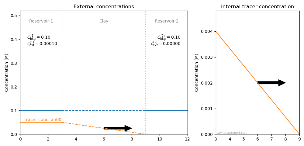
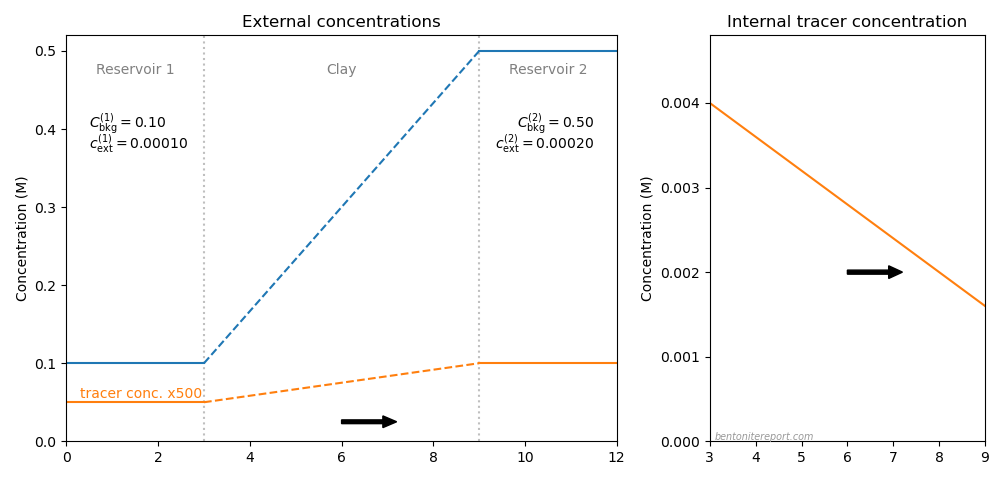
This flaw is well illustrated in examples 2 and 3 in TS15 (the electric potential is the same for these cases). The electric potential in the bulk water can be calculated from the imposed concentration gradients of the main electrolyte, and is plotted in the figure below (blue line)

Here we have chosen \(\Psi_\mathrm{bulk}(0) = 0\) as reference point. (Note that TS15 are under the false impression that \(\Psi_\mathrm{bulk}(x)\) is zero everywhere.)
In the figure is also plotted the electric potential in the “diffuse layer”, as calculated from the Nernst-Planck framework and the concentration profiles in this domain (orange line; also shown here). As we noted previously, the reason for the much smaller variation of \(\Psi_\mathrm{DL}(x)\) as compared with \(\Psi_\mathrm{bulk}(x)\) is the ever-present counter-ions in the “diffuse layer” domain. Notice further that TS15, in contrast, are under the impression that the electrostatic potential in the “diffuse layer” equals the Donnan potential (red line), while such a profound potential variation is not supposed to affect the electromigration, for unclear reasons.
For \(\Psi_\mathrm{DL}\) we have here chosen the reference point \(\Psi_\mathrm{DL}(0) = \Psi^\star(0)\), i.e. we dictate that the bulk and “diffuse layer” potentials should differ by the Donnan potential when \(x=0\). But this is the only point where this condition is fulfilled: The difference between the electric potentials as calculated in this way (green line) does not at all resemble the Donnan potential!
At the moment, I don’t have the energy to sort out if there is any way out of this paradox, but my guess is that the problem is related to the very different treatments of transport in the \(x\)- and \(y\)-directions in the TS15 model. Remember that the assumption of equilibrium between all domains for a given \(x\)-value is equivalent to assuming infinite mobility in the \(y\)-direction of all species. To me, it appears as the TS15 model attempts to squeeze an intrinsically two-dimensional problem into a one-dimensional form. Note that this problem is not unique for the TS15 model, but arise in any multi-porous, multi-component description which assumes local equilibrium between domains (e.g. Appelo and Wersin (2007)).
Appendix: Comments on Figure 8
Disclaimer: This part functions as an appendix to this already appendix-like part of the review. The reader has been warned.
When considering electric potentials in the TS15 model I have developed a need to further comment on “Figure 8”. I alluded to this figure in the previous part of the review when discussing the term “Pseudo 2-D Cartesian system” used by TS15 (a term I don’t understand). “Figure 8” looks like this
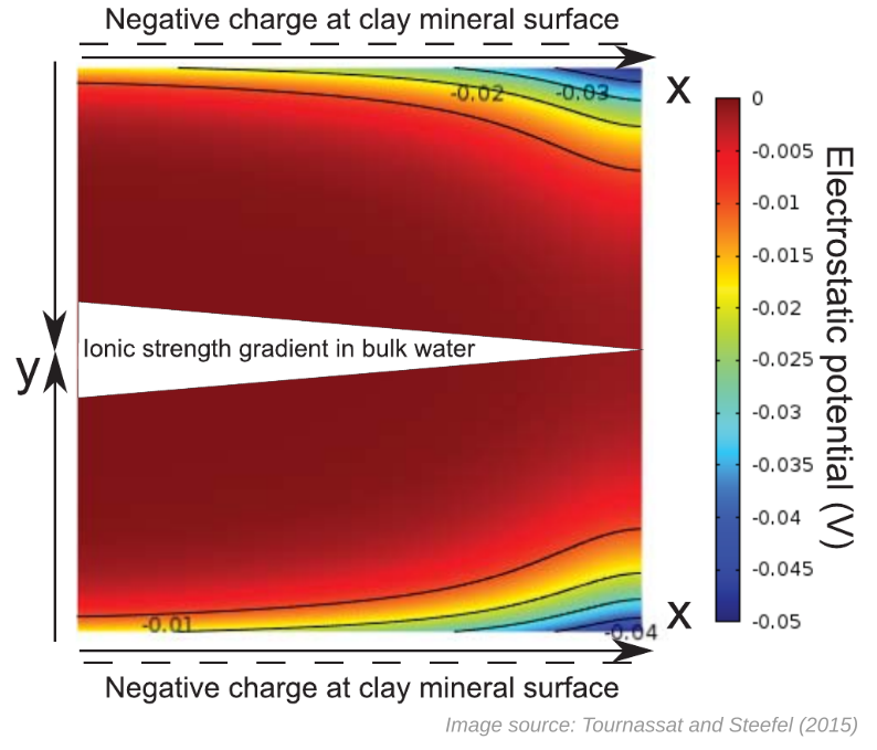
The caption reads
Pseudo-2-D Cartesian system with diffusion along the x-axis and electrostatic potential developing along the y-axis due to the negative charge at clay mineral surfaces.
The only reference to this figure in the article text is at the beginning of the section presenting the transport model (Nernst-Planck equation in several “porosity domains”)
In the following, we will consider a pseudo 2-D Cartesian system in which diffusion takes place along the x axis only (Fig. 8).
The more I think about how this figure is included in the article, the more peculiar I find it. The figure clearly shows a quantitative result, as it displays specific values of a two-dimensional electric potential function outside “negative charge at clay mineral surface”. Yet, any real information about this calculation is nowhere to be found, which I see as a major problem (especially as the text is supposed to be a “fully developed text which can be used for self-study, research, or as a text-book for graduate-level courses”). Here we will first discuss information that is not provided, before continuing with speculating about how this figure may have been produced.
Stuff we are not told anything about
The ionic strength
Note that the “ionic strength gradient in bulk water” is only indicated in the figure, but not at all mentioned in the caption or in the text snippet that refers to this figure. Apparently, the physical situation depicted involves “bulk water” where the ionic strength, i.e. the concentration, falls of with the coordinate \(x\). But what is the actual value of this gradient? What are the boundary concentrations? And how has this ionic strength been used when calculating the electrostatic potential? We are not even told what type of electrolyte is considered! Is it 1:1?
Pseudo-2D and length scales
The only two places in TS15 where “Figure 8” is referenced are also the only places where the concept of a “pseudo-2D Cartesian system” is brought up. But what is meant by this term?! To me, it is more than a little strange to base an entire model presentation on a concept that is not really explained.
Taken at face value, the presented figure does not seem to show any “pseudo-“, but a “real” 2D coordinate system. Guided by the variation of the potential in the \(y\)-direction and by the clue that we are outside a negatively charged mineral surface, it’s quite safe to say that we — in the \(y\)-direction — are looking at an actual diffuse layer, as calculated e.g. in the Gouy-Chapman model. The \(y\)-dimension is thus reasonably on the nanometer scale. An ionic strength gradient, however, only makes sense as being on the macroscopic scale. The scale of the \(x\)-dimension is thus reasonably comparable to e.g. that of a laboratory sample, i.e. centimeters or even meters. Although “Figure 8” consequently is oddly scaled (the \(x\)-dimension is at least a million times larger than the \(y\)-dimension), I don’t see any reason to refer to it as “pseudo-2D”. It should of course be completely mandatory to state the length scales when presenting such a figure in a peer-reviewed scientific journal.
Further, we note that the figure seems to depict two copies facing each other of the same potential function, with one copy being flipped vertically (this explains the two oppositely pointing \(y\)-axes). Is this the reason for calling the coordinate system “Pseudo-2D”? But this manipulation (two copies facing each other) seems only to be for illustrative purposes, and has no impact on what actually seems to have been calculated.4
Surface charge
The potential is supposed to be “developing […] due to the negative charge at the clay mineral surfaces”. But then a surface charge density must have been specified when calculating the potential. Needless to say, this value should have been stated.
Stuff that is incorrect or odd
“Developing” potential
The figure caption “explains” that an electrostatic potential “develop[s] along the \(y\)-axis”. But what is significant is that an electric field is present near the surface. And, as we have brought up earlier, an electric field is equivalent to a potential variation. To put focus on that a potential “develops”, rather than that the potential varies, mostly misses the point. Also, why is the word “develop” used here? It suggests some sort of ongoing (unexplained) process.
“Developing” potential along the y-axis
A clear illustration that something is missed when speaking of potentials rather than fields is that TS15 implies that this “development” occurs exclusively in the \(y\)-direction. Note that an electric field is directed normal to the lines of constant electric potential. It is thus completely clear from the figure itself that the electric field is not in general directed solely in the \(y\)-direction!
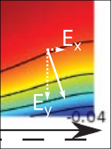
This type of manifestation of an electric field in the \(x\)-direction relates to the complications discussed earlier of having a Donnan potential that varies with \(x\).
The potential has not resulted from solving the Nernst-Planck equation
Even though the purpose of the section is a treatment of the Nernst-Planck framework for transport of ionic charges, “Figure 8” does not present the result of a Nernst-Planck calculation. A main objective of such a treatment is to calculate the gradient of the electric potential (in the \(x\)-direction), i.e. an electric field. In contrast, the figure clearly shows that the potential is essentially zero, some distance away from the surface.
We note that a zero electric potential in the region that the authors presumably classify as “bulk” (some nanometers away from the surface…) is in line with the erroneous procedure of setting the bulk electric potential identically zero in the derivation of the Nernst-Planck flux.
What I think is illustrated/has been calculated
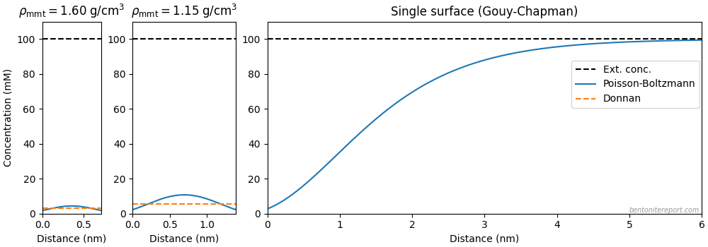
My guess is that “Figure 8” has been produced by calculating a set of potential profiles (in the \(y\)-direction) from the Gouy-Chapaman model for a given set of values of the ionic strength. These profiles have then simply been “stacked” in the \(x\)-direction. Below are some attempts to recreate “Figure 8” using this approach.
Since no parameters are given in TS15, we have to make several assumptions. For the figure below is assumed a linear profile of a 1:1 electrolyte that falls from 1000 mM at \(x=0\) to 100 mM at \(x=12\). We furthermore assume a surface charge density of 0.04 C/m2.
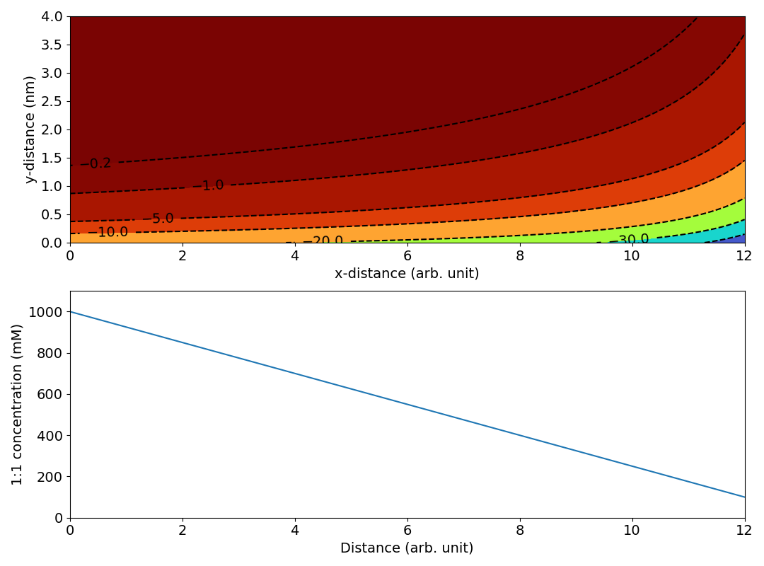
The magnitude and variation of this potential is comparable to that in “Figure 8” (the unit for the electric potential is here mV). We may note, however, that the linear ionic strength profile results in lines of constant electric potential that more and more “bends away” from the surface. This is because the Debye length in a 1:1 electrolyte depends on ionic strength as \(1/\sqrt{I}\). In contrast, the lines of constant potential in “Figure 8” are seen to “bend back”, suggesting a leveling off of the ionic strength, like this
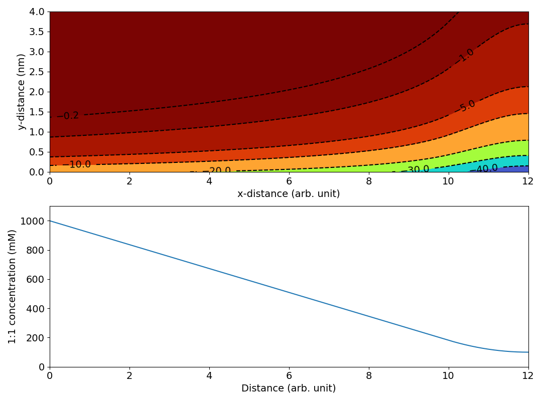
If the present speculations are correct, why on earth has such a concentration profile been chosen? More broadly, why is this type of figure at all presented? If the authors simply want to show the quantities being calculated, why not provide a schematic illustration rather than a quantitative calculation? And if they want to present an actual calculation — which for unclear reasons does not involve the Nernst-Planck framework — they must of course provide a reader with enough information to make it understandable.
Footnotes
[1] As I have commented in the earlier parts: TS15 are fond of using the general terms “clays” and “clay minerals”, while it is clear that the publication mainly focus on systems with substantial ion exchange capacity and swelling properties. Here we will continue to use the term “bentonite” for these systems, and ignore the frequent references in TS15 to more general terms.
[2] TS15 are under the impression that \(\Psi_\mathrm{bulk}= 0\), and they believe that they calculate \(\Psi_\mathrm{DL}\) rather than \(\Psi^\star\). They furthermore emphasize that a more accurate calculation involves integrating the Poisson-Boltzmann equation (and claim falsely that the Donnan equilibrium “model” is based on an approximation of the Poisson-Boltzmann equation). But under all circumstances, the TS15 model requires specifying an arbitrary size of the “diffuse layer”; in the examples is used a width of 3 nm, which approximately corresponds to 3, 1 and 0.3 Debye lengths, respectively, for 1:1 background concentrations 0.1 M, 0.01 M, and 0.001 M. As we have discussed in the blog post on why multi-porosity models cannot be taken seriously, such a partitioning requires that a mechanism is provided for how equilibrium is maintained (i.e. why the “diffuse layer” does not occupy the full pore volume). TS15 do not supply such a mechanism, and neither does any other author promoting multi-porous models.
[3] In this figure, \( \left \{ c_{\mathrm{bulk} ,i} \right \} \) denotes the complete set of imposed concentrations in the bulk water domain. The corresponding set of species concentrations in the “diffuse layer” is denoted \(\left \{ c_{\mathrm{DL},i}\right \}\).
[4] Even if this choice is only “cosmetic”, I actually don’t understand why the figure is presented like this. Is it supposed to depict an (insanely long) interlayer? Perhaps with a “bulk water” phase squeezed in the middle? The same authors have actually presented such types of figures in later publications. As I discuss here, such a representation of a “bulk water” phase is nonsense.


