Category Archives: Homogeneous mixture model

The danger of log-log plots — measuring and modeling “apparent” diffusivity

In a previous blog post, we discussed how the diffusivity of simple cations1 has a small, or even negligible, dependence on background concentration (or, equivalently, on \(K_d\)), and how this observation motivates modeling compacted bentonite as a homogeneous system, containing only interlayer pores.

Despite the indisputable fact that “\(D_a\)”2 for simple ions does not depend much on \(K_d\), the results have seldom been modeled using a homogeneous bentonite model. Instead there are numerous attempts in the bentonite literature to both measure and model a variation of “\(D_a\)” with \(K_d\), usually with a conclusion (or implication) that “\(D_a\)” depends significantly on \(K_d\). In this post we re-examine some of these studies.

The claimed \(K_d\)-dependency is often “supported” by the so-called surface diffusion model. I have previously shown that this model is incorrect.3 Here we don’t concern ourselves with the inconsistencies, but just accept the resulting expression as the model to which authors claim to fit data. This model expression is

\begin{equation} D_a = \frac{D_p + \frac{\rho K_d}{\phi} D_s}{1+\frac{\rho K_d}{\phi}} \tag{1} \end{equation}

where \(D_p\) and \(D_s\) are individual domain diffusivities for bulk water and surface regions, respectively, \(\rho\) is dry density, \(\phi\) porosity, and \(K_d\), of course, is assumed to quantify the distribution of ions between bulk water and surfaces as \(s = K_d\cdot c^\mathrm{bulk}\), where \(s\) is the amount of ions on the surface (per unit dry mass), and \(c^\mathrm{bulk}\) is the corresponding bulk water concentration.

Muurinen et al. (1985)

Muurinen et al. (1985) measured diffusivity in high density bentonite samples at various background concentrations, using a type of closed-cell set-up. They also measured corresponding values of \(K_d\) in batch “sorption” tests. The results for cesium, in samples with density in the range \(1870 \;\mathrm{kg/m^3}\) — \(2030 \;\mathrm{kg/m^3}\), are presented in the article in a figure similar to this:

cesium diffusivivty vs. Kd, model and measurements. From Muurinen et al. (1985)

The markers show experimental data, and the solid curve shows the model (eq. 1) with \(D_p = 1.2 \cdot 10^{-10}\;\mathrm{m^2/s}\)4 and \(D_s = 4.3\cdot 10^{-13}\;\mathrm{m^2/s}\).

The published plot may give the impression of a systematic variation of \(D_a\) for cesium, and that this variation is captured by the model. But the data is plotted with a logarithmic y-axis, which certainly is not motivated. Let’s see how the plot looks with a linear y-axis (we keep the logarithmic x-axis, to clearly see the model variation).

Now the impression is quite different: this way of plotting reveals that the experimental data only cover a part where the model does not vary significantly. With the adopted range on the x-axis (as used in the article) we actually don’t see the full variation of the model curve. Extending the x-axis gives the full picture:

With the full model variation exposed, it is evident that the model fits the data only in a most superficial way. The model “fits” only because it has insignificant \(K_d\)-dependency in the covered range, in similarity with the measurements.

The defining feature of the model is that the diffusivity is supposed to transition from one specific value at high \(K_d\), to a significantly different value at low \(K_d\). As no such transition is indicated in the data, the above “fit” does not validate the model.

Muurinen et al. (1985) also measured diffusion of strontium in two samples of density \(1740 \;\mathrm{kg/m^3}\). The figures below show the data and corresponding model curve.

The left diagram is similar to how the data is presented in the article, while the right diagram utilizes a linear y-axis and shows the full model variation. The line shows the surface diffusion model with parameters \(D_p = 1.2 \cdot 10^{-10}\;\mathrm{m^2/s}\) and \(D_s = 8.8 \cdot 10^{-12}\;\mathrm{m^2/s}\). In this case it is clear even from the published plot that the experimental data shows no significant variation.

The only reasonable conclusion to make from the above data is that cesium and strontium diffusivity does not significantly depend on \(K_d\) (which implies a homogeneous system). This is actually also done in the article:

The apparent diffusivities of strontium and cesium do not change much when the salt concentration used for the saturation of the samples is changed and the sorption factors change. The surface diffusion model agrees fairly well with the observed diffusion-sorption behaviour.

I agree with the first sentence but not with the second. In my mind, the two sentences contradict each other. From the above plots, however, it is trivial to see that the surface diffusion model does not agree (in any reasonable sense) with observations.

Eriksen et al. (1999)

Although Muurinen et al. (1985) concluded insignificant \(K_d\)-dependency on the diffusion coefficients for strontium and cesium, researchers have continued throughout the years to fit the surface diffusion model to experimental data on these and other ions.

Eriksen et al. (1999) present old and new diffusion data for strontium and cesium (and sodium), fitted and plotted in the same way as in Muurinen et al. (1985). Here are the evaluated diffusivities for cesium plotted against evaluated \(K_d\), as presented in the article, and re-plotted in different ways with a linear y-scale:

The curve shows the surface diffusion model (eq. 1), with parameters \(D_p = 8 \cdot 10^{-10}\;\mathrm{m^2/s}\) and \(D_s = 6 \cdot 10^{-13}\;\mathrm{m^2/s}\). The points labeled “Eriksen 99” are original data obtained from through-diffusion tests on “MX-80” bentonite at dry density 1800 \(\mathrm{kg/m^3}\).5 The source for the data points labeled “Muurinen 94” is the PhD thesis of A. Muurinen.6

The upper left plot shows the data as presented in the article; again, a logarithmic y-axis is used. In this case, a zoomed-in view with a linear y-axis (upper right diagram) may still give the impression that the data has a systematic variation that is captured by the model. But viewing the whole range reveals that the model is fitted to data where variation is negligible (bottom diagrams), just as in Muurinen et al. (1985).

Data and model for strontium presented in Eriksen et al. (1999) look like this:

The model (line) has parameters \(D_p = 3 \cdot 10^{-10}\;\mathrm{m^2/s}\) and \(D_s = 1 \cdot 10^{-11}\;\mathrm{m^2/s}\), and the source for the data points labeled “Eriksen 84” is found here.

In this case, not even the diagram presented in the article (left) seems to support the promoted model. This is also confirmed when utilizing a linear y-axis, and showing the full model variation (right diagram).

Eriksen et al. (1999) conclude that strontium diffusivities are basically independent of \(K_d\), but claim, in contrast to Muurinen et al. (1985), that cesium diffusivity depends significantly on \(K_d\):

[I]n the \(K_d\) interval 0.01 to 1 the apparent \(\mathrm{Cs}^+\) diffusivity decreases by approximately one order of magnitude whereas for \(\mathrm{Na}^+\) and \(\mathrm{Sr}^{2+}\) the apparent diffusivity is virtually constant.

They also claim that the surface diffusion model fits the data:

\(D_\mathrm{a}\) curves for \(\mathrm{Cs}^+\) and \(\mathrm{Sr}^{2+}\), calculated using a Eq. (6) [eq. 1 here], are plotted in Fig. 4. As can be seen, good fits to experimental data were obtained […]

Note that the variation in the model for cesium is motivated by three data points with relatively high diffusivity and basically the same \(K_d \sim 0.05\;\mathrm{m^3/kg}\). It seems like the model has been fitted to these points, while the point at \(K_d \sim 0.02\;\mathrm{m^3/kg}\) has been mainly neglected. The resulting model has a huge bulk water diffusivity (\(D_p\)), which is about 7 times larger than in the corresponding fit in Muurinen et al. (1985), and only 2.5 times smaller than the diffusivity for cesium in pure water.

Note that, if you claim that the surface diffusion model fits in this case, you implicitly claim that the observed variation — which still is negligible on the scale of the full model variation — is caused by the influence of this enormous (for a 1800 \(\mathrm{kg/m^3}\) sample) bulk pore water diffusivity; with a more “reasonable” value for \(D_p\), the model no longer fits. There are consequently valid reasons to doubt that the claimed \(K_d\) dependence is real. We will return to this fit in the next section.

Gimmi & Kosakowski (2011)

We have now seen several examples of authors erroneously claiming (or implying) that a surface diffusion model is valid, when the actual data for “\(D_a\)” has no significant \(K_d\)-dependency. For reasons I cannot get my head around, this flawed treatment is still in play.

Rather than identifying the obvious problem with the previously presented fits, Gimmi and Kosakowski (2011) instead extended the idea of expressing the diffusivity as a function of \(K_d\) by using scaled, dimensionless quantities

\begin{equation} D_\mathrm{arw} = \frac{D_\mathrm{a}\tau_w}{D_0} \tag{2} \end{equation}

\begin{equation} \kappa = \frac{\rho K_d}{\phi} \end{equation}

where \(D_0\) is the corresponding diffusivity in pure water and \(\tau_w\) is the “tortuosity factor” for water in the system of interest. This factor is simply the ratio between the water diffusivity in the system of interest and the water diffusivity in pure water (I have written about the problem with factors like this here).

The idea — it seems — is that using \(D_\mathrm{arw}\) and \(\kappa\) as variables should make it possible to directly compare the mobility of a given species in systems differing in density, clay content, etc.

Even though it makes some sense that the diffusivity of a specific species scales with the diffusivity of water in the same system, the above procedure inevitably introduces more variation in the data — both because an additional measured quantity (water diffusivity) is involved when evaluating the scaled diffusivity, but also because water diffusivity may depend differently on density as compared with the diffusivity of the species under study.

Also Gimmi and Kosakowski (2011) use the flawed surface diffusion model for analysis, and their expression for \(D_\mathrm{arw}\) is

\begin{equation} D_\mathrm{arw} = \frac{1+\mu_s\kappa}{1+\kappa} \tag{3} \end{equation}

where \(\mu_s = D_s\tau_w/D_0\) is a “relative surface mobility”. This equation is obtained from eq. 1, by dividing by \(D_p\) and assuming \(D_p = D_0/\tau_w\).

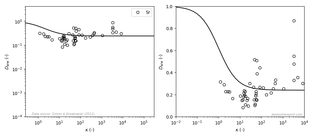
Gimmi and Kosakowski (2011) fit eq. 3 to a large set of collected data, measured in various types of material, including bentonites, clay rocks, and clayey soils. This is their result for cesium7 (the model curve is eq. 3 with \(\mu_s = 0.031\)8)

Viewed as a whole, this data is more scattered as compared with the previous studies. This is reasonably an effect of the larger diversity of the samples, but also an effect of multiplying the “raw” diffusion coefficient with the factor \(\tau_w\) (eq. 2).

Just as in the previous studies we have looked at, the published plot (similar to the left diagram) may give the impression of a systematic variation of the diffusivity with \(K_d\) (it contains partly the same data). But just as before, a linear y-axis (right diagram) reveals that the model is fitted only to data where variation is negligible.

Note that the three data points that contributed to the majority of the variation in the fitted model in Eriksen et al. (1999) here appear as outliers.9 The variation with \(K_d\) for cesium claimed in that study is thus invalidated by this larger data set.

As we have noted already, the only reasonable conclusion to draw from this data is that there is no systematic \(K_d\)-dependency on diffusivity of cesium or strontium, and that it does not — in any reasonable sense — fit the surface diffusion model. Yet, also Gimmi and Kosakowski (2011) imply that the surface diffusion is valid:

The data presented here show a general agreement with a simple surface diffusion model, especially when considering the large errors associated with the \(D_\mathrm{erw}\) and \(D_\mathrm{arw}\).

This paper, however, contains an even worse “fit” to strontium data, as compared to the earlier studies (the left diagram is similar to the how it is presented in the article, the right diagram uses a linear y-axis; the line is eq. 3 with \(\mu_s = 0.24\)8):

This data does not suggest a variation in accordance with the adopted model even when plotted in a log-log diagram. With a linear y-axis, the dependence rather seems to be the opposite: \(D_\mathrm{arw}\) appears to increase with \(\kappa\). However, I suspect that this is a not a “real” dependence, but rather an effect of trying to construct a “relative” diffusivity; note that while \(\kappa\) spans four orders of magnitude, \(D_\mathrm{arw}\) scatters only by a factor of 5 or 6. Nevertheless, how this data can be claimed to show “general agreement” with the surface diffusion model is a mystery to me.

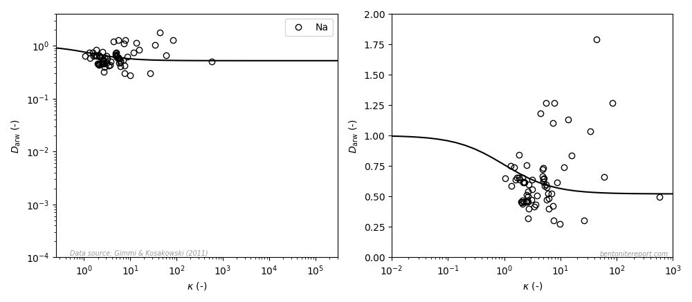
The view is similar for sodium (the left diagram is similar to the how it is presented in the article, the right diagram uses a linear y-axis; the line is eq. 3 with \(\mu_s=0.52\)8):

Even if the model in this case only displays minor variation, it can hardly be claimed to fit the data: again, the data suggests a diffusivity that increases with \(\kappa\). But a significant amount of these data points have \(D_\mathrm{arw} > 1\), which is not likely to be true, as it indicates that the relative mobility for sodium is larger than for water. Consequently, the major contribution of the variation seen in this data is most probably noise.

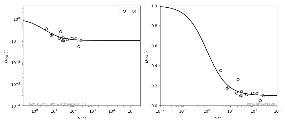
Gimmi and Kosakowski (2011) also examined diffusivity for calcium, and the data looks like this (the left diagram is similar to the how it is presented in the article, the right diagram uses a linear y-axis; the line is eq. 3 with \(\mu_s=0.1\)8):

Here it looks like the data, to some extent, behaves in accordance with the model also when plotted with linear y-axis covering the full model variation. However, there are significantly less data reported for calcium (as compared with cesium, strontium, and sodium) and the model variation is supported only by a few data points10. I therefore put my bet on that if calcium diffusivity is studied in more detail, the dependence suggested by the above plot will turn out to be spurious.11

Some thoughts

I am more than convinced that the only reasonable starting point for modeling saturated bentonite is a homogeneous description. I had nevertheless expected to at least have to come up with an argument against the multi-porous view put forward in the considered publications (and in many others). I am therefore quite surprised to find that this argument is already provided by the data in the very same publications (and even by the statements, sometimes): there is nothing in the data here reviewed that seriously suggests that cation diffusion is influenced by a heterogeneous pore structure.

Still, the unsupported idea that cations in compacted bentonite are supposed to diffuse in two (or more) different types of water domains has evidently propagated through the scientific literature for decades, and a multi-porous view is mainstream in modern bentonite research. It is difficult to not feel disheartened when faced with this situation. What would it take for researchers to begin scrutinize their assumptions? Is nobody interested in the topics we are supposed to study?

Footnotes

[1] Unfortunately, a quantity which by many is incorrectly interpreted as an “apparent” diffusivity.

[2] I use quotation marks to indicate that \(D_a\) is a parameter in the traditional diffusion-sorption model, a model not valid for compacted bentonite. Still, this parameter is often reported as if it was a directly measured quantity.

[3] I have also derived a correct version of the surface diffusion model, which does not involve apparent diffusivity.

[4] The article states \(\epsilon D_p = 3.5\cdot 10^{-11}\; \mathrm{m^2/s}\), where \(\epsilon\) is the porosity. \(D_p = 1.2\cdot 10^{-10} \; \mathrm{m^2/s}\) corresponds to \(\epsilon = 0.29\).

[5] In this study, both \(K_d\) and \(D_a\) were evaluated by fitting the traditional diffusion-sorption model to concentration measurements.

[6] I have had no access to this document, and I have not verified e.g. sample density (this data set is different from that presented in the previous section). Instead, I have read these values from the diagram in Eriksen et al. (1999).

[7] They actually divide their cesium data into two categories, which show quite different mobility. The data shown here — which includes bentonite samples — is for systems categorized as being “non-illite” or having Cs concentration above “trace”.

[8] According to the article table, the fitted values for \(\mu_s\) are 0.52 (Na), 0.39 (Sr), 0.087 (Ca), and 0.015 (Cs). The plotted lines, however, appear to instead use what is listed as “mean \(\mu_s\)”. Here, I have used these \(\mu_s\)-values: 0.52 (Na), 0.24 (Sr), 0.1 (Ca), and 0.031 (Cs).

[9] This cluster contains a fourth data point, from Jensen and Radke (1988).

[10] All data for calcium is essentially from only two different sources: Staunton (1990) and Oscarsson (1994).

[11] It would also be more than amazing if it turns out — after it is verified that Cs, Na, and (especially) Sr show no significant \(K_d\) dependence — that Ca diffusivity actually varies in accordance with the flawed surface-diffusion model!

Donnan equilibrium and the homogeneous mixture model

We can directly apply the homogeneous mixture model for bentonite to isolated systems — e.g. closed-cell diffusion tests — as discussed previously. For systems involving external solutions we must also handle the chemical equilibrium at solution/bentonite interfaces.

I have presented a framework for calculating the chemical equilibrium between an external solution and a bentonite component in the homogeneous mixture model here. In this post I will discuss and illustrate some aspects of that work.

Overview

We assume a homogeneous bentonite domain in contact with an external solution, with the clay particles prevented from crossing the domain interface. For real systems, this corresponds to the frequently encountered set-up with bentonite confined in a sample holder by means of e.g. a metal filter. From the assumptions of the homogeneous model — that all ions are mobile and allowed to cross the domain interface — it follows that the type of equilibrium to consider is the famous Donnan equilibrium. I have discussed the Donnan effect and its relevance for bentonite quite extensively here.

Since the adopted model assumes a homogeneous bentonite domain, the only region where Donnan equilibrium comes into play is at the interface between the bentonite and the external solution. This is quite different from how Donnan equilibrium calculations are implemented in many multi-porous models, where the equilibrium is internal to the clay — between assumed “macro” and “micro” compartments of the pore structure. The need for performing Donnan equilibrium calculations is thus minimized in the homogeneous mixture model (as mentioned, isolated systems require no such calculations). Note also that the semi-permeable mechanism in multi-porous models is required to act on the pore-scale. I have never seen any description or explanation how such a mechanism is supposed to work.1 In the homogeneous mixture model, on the other hand, the semi-permeable interface corresponds directly to a macroscopic and experimentally well-defined component: the confining filter.

The problem to be solved can be illustrated like this

Schematic illustration of an external solution in contact with a homogeneous bentonite domain

The aim is to relate the set of species concentrations in the external solution (\(\{c_i^\mathrm{ext}\}\)) to those in the clay domain (\(\{c_i^\mathrm{int}\}\)) when the system is in equilibrium. This is done by applying the standard approach to Donnan equilibrium, as found in textbooks on the subject. If there is anything “radical” about this framework, it is thus not in the way Donnan equilibrium is implemented, but rather in treating bentonite as a single phase: this approach is formally equivalent to assuming the bentonite to be an aqueous solution.

Chemical equilibrium

I prefer to formulate the Donnan equilibrium framework in a way that separates effects due to difference in the local chemical environment from effects due to differences in electrostatic potential between the two compartments. An important reason for focusing on this separation is that the local environment affects the chemistry under all circumstances, while the (relative) value of the electrostatic potential only is relevant when bentonite is contacted with an external solution. We therefore express the chemical equilibrium as

\begin{equation} \frac{c_i^\mathrm{int}}{c_i^\mathrm{ext}} = \frac{\gamma_i^\mathrm{ext}}{\gamma_i^\mathrm{int}}\cdot e^{-\frac{z_iF\psi^\star}{RT}} \tag{1} \end{equation}

This formula is achieved by setting the electro-chemical potential equal for each species in the two compartments. Here \(\gamma_i\) denotes the activity coefficient for species \(i\), and \(\psi^*\) is the electrostatic potential difference between the compartments, which we refer to as the Donnan potential.

I find it convenient to rewrite this expression using some fancy Greek letters

\begin{equation} \label{eq:chem_eq2} \Xi_i = \Gamma_i \cdot f_D^{-z_i} \tag{2} \end{equation}

Here I call \(\Xi_i = c_i^\mathrm{int}/c_i^\mathrm{ext}\) the ion equilibrium coefficient for species \(i\). This quantity expresses the essence of ion equilibrium in the homogeneous mixture model, and will appear in many places in the analysis. \(\Xi_i\) has two factors:

  • \(\Gamma_i = \gamma_i^\mathrm{ext}/\gamma_i^\mathrm{int}\) expresses the chemical aspect of the equilibrium: when \(\Gamma_i\) is large (\(>1\)), the species has a chemical preference for residing in the interlayer pores, and when \(\Gamma_i\) is small (\(<1\)), the species has a preference for the external solution. In general, \(\Gamma_i\) for any specific species \(i\) is a function of all species concentrations in the system.
  • \(f_D^{-z_i}\), where \(f_D = e^{\frac{F\psi^\star}{RT}}\) is a dimensionless transformation of the Donnan potential (this is basically the Nernst equation), which we here call the Donnan factor. \(f_D\) expresses the electrostatic aspect of the equilibrium, and is the same for all species. The effect on \(\Xi_i\), however, is different for species of different charge number, because of the exponent \(-z_i\) in the full expression.

I want to emphasize that eqs. 1 and 2 express the exact same thing: chemical equilibrium between the two compartments.

Illustrations

To get a feel for the quantity \(\Xi\), here is a hopefully useful animation

Relation beteween internal and external concentration for varying Xi

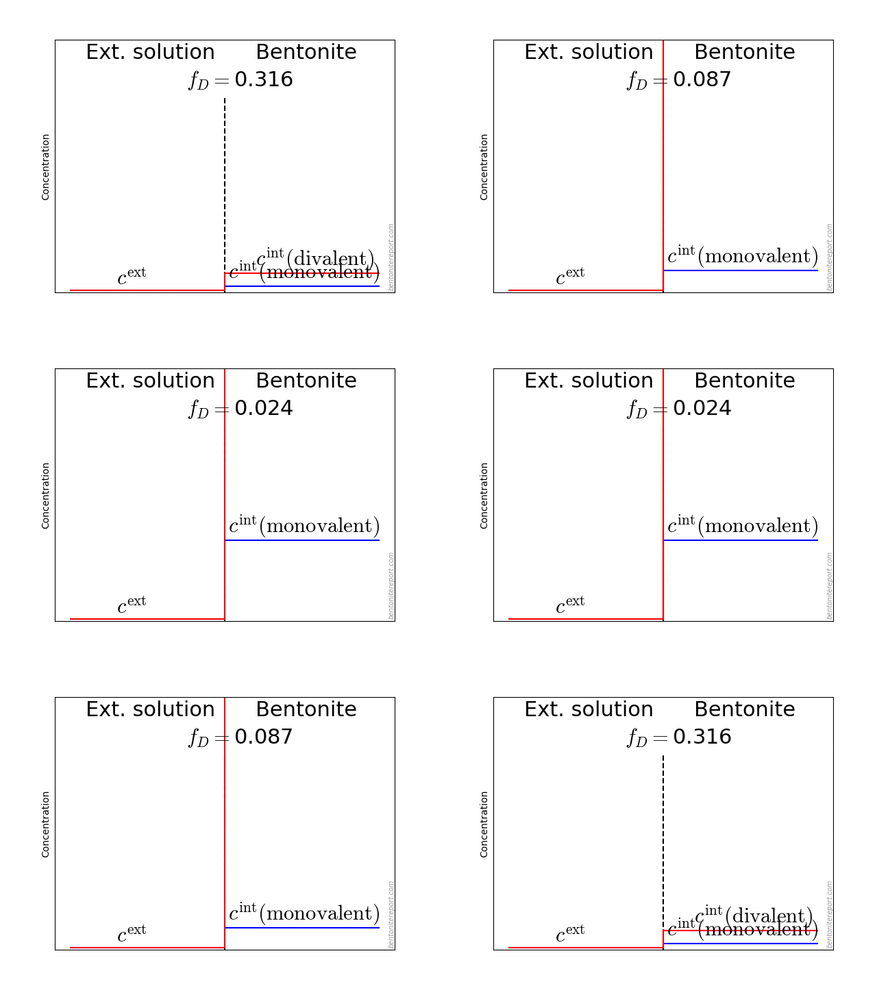
It may also be helpful to see the influence of \(f_D\) on the equilibrium. Since the Donnan potential is negative, \(f_D\) is less than unity and typical values in relevant bentonite systems is \(f_D \sim\) 0.01 — 0.4. Due to the exponent \(-z_i\) in eq. 2, this influence on the equilibrium looks quite different for species with different valency. For mono- and di-valent cations, the behavior looks like this (here is put \(\Gamma = 1\) for both species)

Variation of internal cation concentrations with varying Donnan factor

The typical behavior for cations is that the internal concentration is much larger than the corresponding external concentration (at \(f_D = 0.01\) in the above animation, the internal concentration for the di-valent cation is enhanced by a factor \(\Xi = 10 000\)!). For anions, the internal concentration is instead lower than the external concentration,2 as shown here (\(\Gamma = 1\) for both species)

Variation of internal anion concentration with the Donnan factor

Equation for \(f_D\)

For a complete description, we need an equation for calculating \(f_D\). This is derived by requiring charge neutrality in the two compartments and looks like

\begin{equation*} \sum_i z_i\cdot\Gamma_i \cdot c_i^\mathrm{ext} \cdot f_D^{-z_i} – c_{IL} = 0 \tag{3} \end{equation*}

where

\begin{equation*} c_{IL} = \frac{CEC}{F \cdot w} \end{equation*}

is the structural charge present in the clay (i.e. negative montmorillonite layer charge) expressed as a monovalent interlayer concentration. Here \(CEC\) is the cation exchange capacity of the clay component, \(w\) the water-to-solid mass ratio,3 and \(F\) is the Faraday constant.

The way eq. 3 is formulated implies that the external concentrations should be used as input to the calculation. This is typically the case as the external concentrations are under experimental control.

In typical geochemical systems it is required to account for aqueous species with valency at least in the range -2 — +2 (e.g. \(\mathrm{Ca}^{2+}\), \(\mathrm{Na}^{+}\), \(\mathrm{Cl}^{-}\), \(\mathrm{SO_4}^{2-}\)), which implies that the equation for calculating \(f_D\) is generally a polynomial equation of degree four or higher.

An important special case is the 1:1 system — e.g. pure Na-montmorillonite contacted with a NaCl solution — which has an equation for \(f_D\) of only degree two, and thus has a relatively simple analytical solution

\begin{equation*} f_D = \frac{c_{IL}}{2c^\mathrm{ext} \Gamma_\mathrm{Cl}} \left ( \sqrt{1+ \frac{4(c^\mathrm{ext})^2 \Gamma_\mathrm{Na}\Gamma_\mathrm{Cl}} {c_{IL}^2}} – 1 \right ) \end{equation*}

With the machinery in place for calculating the Donnan potential, here is an animation demonstrating the response in internal sodium and chloride concentrations as the external NaCl concentration is varied. In this calculation \(c_{IL} = 2\) M, and \(\Gamma_\mathrm{Na} = \Gamma_\mathrm{Cl} = 1\)

Relation between internal and external Na and Cl concentrations

Comment on through-diffusion

To me, the last illustration makes it absolutely clear that Donnan equilibrium and the homogeneous mixture model provide the correct principal explanation for e.g. the behavior of tracer ions in through-diffusion tests. If you choose to relate the flux in through-diffusion tests to the external concentration difference — which is basically done in all published studies, via the parameter \(D_e\) — you will evaluate large “diffusivities” for cations and small “diffusivities” for anions. These “diffusivities” will, moreover, have the opposite dependence on background concentration: the cation flux diverges in the low background concentration limit,4 while the anion flux approaches zero.

But this behavior is seen to be caused by differently induced internal concentration gradients. If fluxes are related to these gradients — which they of course should, if you strive for an actual Fickian description — you find that the diffusivities are no different from what is evaluated in closed-cell tests. Relating the steady-state flux to the external concentration difference in the homogeneous mixture model gives (assuming zero tracer concentration on the outflow side)

\begin{equation*} j_\mathrm{ss} = -\phi\cdot D_c \cdot \nabla c^\mathrm{int} = \phi\cdot D_c \cdot\Xi\cdot \frac{c^\mathrm{source}}{L} \end{equation*}

where \(c^\mathrm{source}\) denotes the tracer concentration in the external solution on the inflow side, \(\phi\) is the porosity, \(D_c\) is the pore diffusivity in the interlayer domain, and \(L\) is the length of the bentonite sample. From the above equation can directly be identified

\begin{equation} D_e = \phi\cdot\Xi\cdot D_c \end{equation}

\(D_e\) is thus not a diffusion coefficient, but basically a measure of \(\Xi\).

Note that this explanation for the behavior of \(D_e\) does not invoke any notion of an anion accessible volume, nor any “sorption” concept for cations.5

Additional comments

When I first published on Donnan equilibrium in bentonite, I was a bit confused and singled out the term “Donnan equilibrium” to refer to anions only, while calling the corresponding cation equilibrium “ion-exchange equilibrium”. To refer to “both” types of equilibrium we used the term “ion equilibrium”.6 Of course, Donnan equilibrium applies to ions of any charge and, being better informed, I should have used a more stringent terminology. In later publications I have tried to make amends by pointing out that the process of cation exchange is part of the establishment of Donnan equilibrium.

Being new to the Donnan equilibrium world, I also invented some of my own nomenclature and symbols: e.g. I named the ratio between internal and external concentration the ion equilibrium coefficient (\(\Xi\)). Conventionally, if I now have understood correctly, this concentration ratio is referred to as the “Donnan ratio”, and is usually labeled \(r\) (although I’ve also seen \(K\)).

But the term “Donnan ratio” seems to be used slightly differently in different contexts, e.g. defined either as \(c^\mathrm{int}/c^\mathrm{ext}\) or as \(c^\mathrm{ext}/c^\mathrm{int}\), and is sometimes related more directly to the Donnan potential (if no distinction is made between activities and concentrations, we can write \(f_D^{-z_i} = c_i^\mathrm{int}/c_i^\mathrm{ext}\)). I therefore will continue to use the term “ion equilibrium coefficient” — with label \(\Xi\) — in the context of bentonite systems. This usage has also been picked up in some other clay publications. The ion equilibrium coefficient should be understood as strictly defined as \(\Xi = c^\mathrm{int}/c^\mathrm{ext}\) for any species, and never to define, or being defined by, the Donnan potential.

To emphasize the difference between effects due to the presence of a Donnan potential and effects due to different local chemical environments, I will refer to \(f_D\) as the Donnan factor. (This term does not seem to be used conventionally for any other quantity, although there are examples where it is used as a synonym for Donnan ratio.)

Finally, as in any other approach, the current framework requires a description for the activity coefficients. For activity coefficients in the external solution, there are quite a number of models already available. For the interlayer, modeling — and measuring! — activities is an open research area (at least I hope that this research area is open).

Footnotes

[1] This is just one of several major “loose ends” in most multi-porous models. I have earlier discussed the lack of treatment of swelling, and the incorrect treatment of fluxes in different domains. Update (220622): The lack of a semi-permeable component in multi-porosity models is further discussed here.

[2] This does not have to be the case in principle, if \(\Gamma\) for the anion is large, at the same time as the external concentration is not too low.

[3] Hence, it is implied that we use concentration units based on water mass (molality).

[4] What actually happens is that the transport resistance in the filters begins to dominate.

[5] Speaking of “sorption”, we have noted before that this term nowadays is used to mean any type of uptake between bulk water and some other domain (where the species may or may not be immobile). In this sense, there is “sorption” in the homogeneous mixture model (for both cations and anions), but only at interfaces to external solutions. It thus translates to a boundary condition, rather than being part of the transport dynamics within the clay (which makes life much simpler from a numeric perspective). Update (220622): The homogeneous mixture model is extended to deal with ions that truly sorbs here.

[6] It turns out Donnan himself actually used this terminology (“ionic equilibria”)

Sorption part II: Letting go of the bulk water

Disclaimer: The following discussion applies fully to ions that only interact with bentonite by means of being part of an electric double layer. Here such ions are called “simple” ions. Species with more specific chemical interactions will be discussed in separate blog posts.

The “surface diffusion” model is not suitable for compacted bentonite

In the previous post on sorption1 we derived a correct “surface diffusion” model. The equation describing the concentration evolution in such a model is a real Fick’s second law, meaning that it only contains the actual diffusion coefficient (apart from the concentration itself)

\begin{equation}
\frac{\partial c}{\partial t} = D_\mathrm{sd} \cdot\nabla^2 c \tag{1}
\end{equation}

Note that \(c\) in this equation still denotes the concentration in the presumed bulk water,2 while \(D_\mathrm{sd}\) relates to the mobility, on the macroscopic scale, of a diffusing species in a system consisting of both bulk water and surfaces.3

Conceptually, eq. 1 states that there is no sorption in a surface diffusion model, in the sense that species do not get immobilized. Still, the concept of sorption is frequently used in the context of surface diffusion, giving rise to phrases such as “How Mobile Are Sorbed Cations in Clays and Clay Rocks?”. The term “sorption” has evidently shifted from referring to an immobilization process, to only mean the uptake of species from a bulk water domain to some other domain (where the species may or may not be mobile). In turn, the role of the parameter \(K_d\) is completely shifted: in the traditional model it quantifies retardation of the diffusive flux, while in a surface diffusion model it quantifies enhancement of the flux (in a certain sense).

A correct4 surface diffusion model resolves several of the inconsistencies experienced when applying the traditional diffusion-sorption model to cation diffusion in bentonite. In particular, the parameter referred to as \(D_e\) may grow indefinitely without violating physics (because it is no longer a real diffusion coefficient), and the insensitivity of \(D_\mathrm{sd}\) to \(K_d\) may be understood because \(D_\mathrm{sd}\) is the real diffusion coefficient (it is not an “apparent” diffusivity, which is expected to be influenced by a varying amount of immobilization).

Still, a surface diffusion model is not a very satisfying description of bentonite, because it assumes the entire pore volume to be bulk water. To me, it seems absurd to base a bentonite model on bulk water, as the most characteristic phenomenon in this material — swelling — relies on it not being in equilibrium with a bulk water solution (at the same pressure). It is also understood that the “surfaces” in a surface diffusion model correspond to montmorillonite interlayer spaces — here defined as the regions where the exchangeable ions reside5 — which are known to dominate the pore volume in any relevant system.

Indeed, assuming that diffusion occurs both in bulk water and on surfaces, it is expected that \(D_\mathrm{sd}\) actually should vary significantly with background concentration, because a diffusing ion is then assumed to spend considerably different times in the two domains, depending on the value of \(K_d\).6

Using the sodium diffusion data from Tachi and Yotsuji (2014) as an example, \(\rho\cdot K_d\) varies from \(\sim 70\) to \(\sim 1\), when the background concentration (NaCl) is varied from 0.01 M to 0.5 M (at constant dry density \(\rho=800\;\mathrm{kg/m^3}\)). Interpreting this in terms of a surface diffusion model, a tracer is supposed to spend about 1% of the time in the bulk water phase when the background concentration is 0.01 M, and about 41% of the time there when the background concentration is 0.5 M7. But the evaluated values of \(D_\mathrm{sd}\) (referred to as “\(D_a\)” in Tachi and Yotsuji (2014)) show a variation less than a factor 2 over the same background concentration range.

Insignificant dependence of \(D_\mathrm{sd}\) on background concentration is found generally in the literature data, as seen here (data sources: 1, 2, 3, 4, 5)

Diffusion coefficients as a function of background concentration for Sr, Cs, and Na.

These plots show the deviation from the average of the macroscopically observed diffusion coefficients (\(D_\mathrm{macr.}\)). These diffusion coefficients are most often reported and interpreted as “\(D_a\)”, but it should be clear from the above discussion that they equally well can be interpreted as \(D_\mathrm{sd}\). The plots thus show the variation of \(D_\mathrm{sd}\), in test series where \(D_\mathrm{sd}\) (reported as “\(D_a\)”) has been evaluated as a function of background concentration.8 The variation is seen to be small in all cases, and the data show no systematic dependencies on e.g. type of ion or density (i.e., at this level of accuracy, the variation is to be regarded as scatter).

The fact that \(D_\mathrm{sd}\) basically is independent of background concentration strongly suggests that diffusion only occurs in a single domain, which by necessity must be interlayer pores. This conclusion is also fully in line with the basic observation that interlayer pores dominate in any relevant system.

Diffusion in the homogeneous mixture model

A more conceptually satisfying basis for describing compacted bentonite is thus a model that assigns all pore volume to the surface regions and discards the bulk water domain. I call this the homogeneous mixture model. In its simplest version, diffusive fluxes in the homogeneous mixture model is described by the familiar Fickian expression

\begin{equation} j = -\phi\cdot D_c \cdot \nabla c^\mathrm{int} \tag{2} \end{equation}

where the concentration of the species under consideration, \(c^\mathrm{int}\), is indexed with an “int”, to remind us that it refers to the concentration in interlayer pores. The corresponding diffusion coefficient is labeled \(D_c\). Notice that \(c^\mathrm{int}\) and \(D_c\) refer to macroscopic, averaged quantities; consequently, \(D_c\) should be associated with the empirical quantity \(D_\mathrm{macr.}\) (i.e. what we interpreted as \(D_\mathrm{sd}\) in the previous section, and what many unfortunately interpret as \(D_a\)) — \(D_c\) is not the short scale diffusivity within an interlayer.

For species that only “interact” with the bentonite by means of being part of an electric double layer (“simple” ions), diffusion is the only process that alters concentration, and the continuity equation has the simplest possible form

\begin{equation} \frac{\partial n}{\partial t} + \nabla\cdot j = 0 \end{equation}

Here \(n\) is the total amount of diffusing species per volume porous system, i.e. \(n = \phi c^\mathrm{int}\). Inserting the expression for the flux in the continuity equation we get

\begin{equation} \frac{\partial c^\mathrm{int}}{\partial t} = D_c \cdot \nabla^2 c^\mathrm{int} \tag{3} \end{equation}

Eqs. 2 and 3 describe diffusion, at the Fickian level, in the homogeneous mixture model for “simple” ions. They are identical in form to the Fickian description in a conventional porous system; the only “exotic” aspect of the present description is that it applies to interlayer concentrations (\(c^\mathrm{int}\)), and more work is needed in order to apply it to cases involving external solutions.

But for isolated systems, e.g. closed-cell diffusion tests, eq. 3 can be applied directly. It is also clear that it will reproduce the results of such tests, as the concentration evolution is known to obey an equation of this form (Fick’s second law).

Model comparison

We have now considered three different models — the traditional diffusion-sorption model, the (correct) surface diffusion model, and the homogeneous mixture model — which all can be fitted to closed-cell diffusion data, as exemplified here

three models fitted to diffusion data for Sr from Sato et al. (92)

The experimental data in this plot (from Sato et al. (1992)) represent the typical behavior of simple ions in compacted bentonite. The plot shows the resulting concentration profile in a Na-montmorillonite sample of density 600 \(\mathrm{kg/m^3}\), where an initial planar source of strontium, embedded in the middle of the sample, has diffused for 7 days. Also plotted are the identical results from fitting the three models to the data (the diffusion coefficient and the concentration at 0 mm were used as fitting parameters in all three models).

From the successful fitting of all the models it is clear that bentonite diffusion data alone does not provide much information for discriminating between concepts — any model which provides a governing equation of the form of Fick’s second law will fit the data. Instead, let us describe what a successful fit of each model implies conceptually

  • The traditional diffusion-sorption model

    The entire pore volume is filled with bulk water, in contradiction with the observation that bentonite is dominated by interlayer pores. In the bulk water strontium diffuse at an unphysically high rate. The evolution of the total ion concentration is retarded because most ions sorb onto surface regions (which have zero volume) where they become immobilized.

  • The “surface diffusion” model

    The entire pore volume is filled with bulk water, in contradiction with the observation that bentonite is dominated by interlayer pores. In the bulk water strontium diffuse at a reasonable rate. Most of the strontium, however, is distributed in the surface regions (which have zero volume), where it also diffuse. The overall diffusivity is a complex function of the diffusivities in each separate domain (bulk and surface), and of how the ion distributes between these domains.

  • The homogeneous mixture model

    The entire pore volume consists of interlayers, in line with the observation that bentonite is dominated by such pores. In the interlayers strontium diffuse at a reasonable rate.

From these descriptions it should be obvious that the homogeneous mixture model is the more reasonable one — it is both compatible with simple observations of the pore structure and mathematically considerably less complex as compared with the others.

The following table summarizes the mathematical complexity of the models (\(D_p\), \(D_s\) and \(D_c\) denote single domain diffusivities, \(\rho\) is dry density, and \(\phi\) porosity)

Summary models

Note that the simplicity of the homogeneous mixture model is achieved by disregarding any bulk water phase: only with bulk water absent is it possible to describe experimental data as pure diffusion in a single domain. This process — pure diffusion in a single domain — is also suggested by the observed insensitivity of diffusivity to background concentration.

These results imply that “sorption” is not a valid concept for simple cations in compacted bentonite, regardless of whether this is supposed to be an immobilization mechanism, or if it is supposed to be a mechanism for uptake of ions from a bulk water to a surface domain. For these types of ions, closed-cell tests measure real (not “apparent”) diffusion coefficients, which should be interpreted as interlayer pore diffusivities (\(D_c\)).

Footnotes

[1] Well, the subject was rather on “sorption” (with quotes), the point being that “sorbed” ions are not immobilized.

[2] Eq. 1 can be transformed to an equation for the “total” concentration by multiplying both sides by \(\left (\phi + \rho\cdot K_d\right)\).

[3] Unfortunately, I called this quantity \(D_\mathrm{macr.}\) in the previous post. As I here compare several different diffusion models, it is important to separate between model parameters and empirical parameters, and the diffusion coefficient in the “surface diffusion” model will henceforth be called \(D_\mathrm{sd}\). \(D_\mathrm{macr.}\) is used to label the empirically observed diffusion parameter. Since the “surface diffusion” model can be successfully fitted to experimental diffusion data, the value of the two parameters will, in the end, be the same. This doesn’t mean that the distinction between the parameters is unimportant. On the contrary, failing to separate between \(D_\mathrm{macr.}\) and the model parameter \(D_\mathrm{a}\) has led large parts of the bentonite research community to assume \(D_\mathrm{a}\) is a measured quantity.

[4] It might seem silly to point out that the model should be “correct”, but the model which actually is referred to as the surface diffusion model in the literature is incorrect, because it assumes that diffusive fluxes in different domains can be added.

[5] There is a common alternative, implicit, and absurd definition of interlayer, based on the stack view, which I intend to discuss in a future blog post. Update (220906): This interlayer definition and stacks are discussed here.

[6] Note that, although \(D_\mathrm{sd}\) is not given simply by a weighted sum of individual domain diffusivities in the surface diffusion model, it is some crazy function of the ion mobilities in the two domains.

[7] With this interpretation, the fraction of bulk water ions is given by \(\frac{\phi}{\phi+\rho K_d}\).

[8] The plot may give the impression that such data is vast, but these are basically all studies found in the bentonite literature, where background concentration has been varied systematically. Several of these use “raw” bentonite (“MX-80”), which contains soluble minerals. Therefore, unless this complication is identified and dealt with (which it isn’t), the background concentration may not reflect the internal chemistry of the samples, i.e. the sample and the external solution may not be in full chemical equilibrium. Also, a majority of the studies concern through-diffusion, where filters are known to interfere at low ionic strength, and consequently increase the uncertainty of the evaluated parameters. The “optimal” tests for investigating the behavior of \(D_\mathrm{macr.}\) with varying background concentrations are closed-cell tests on purified montmorillonite. There are only two such tests reported (Kozaki et al. (2008) and Tachi and Yotsuji (2014)), and both are performed on quite low density samples.