After developing a tool that solves the 1-dimensional Nernst-Planck equations in bentonite, we have explored some possible consequences of electromigration. For an introduction to multi-component diffusion in bentonite, and definitions of various electric potentials, et.c., we refer to the latest installment in the series on semi-permeability. We have noted that diffusion potentials in bentonite diffusion tests can be quite small in several cases, due to the ever-present exchangeable cations, which provide a way to effectively erase any electric current caused by differences in mobility of different types of ions. The diffusion potential in the model of the “uphill” test is only 0.06 mV, and even for pure CaCl2 diffusion with \(c_\mathrm{IL}\) = 3.0 M, the modeled diffusion potential is only about 1 mV. In the examples of Tournassat and Steefel (2015), we also evaluated a diffusion potential of 1.0 mV.
In cases with substantial amounts of different types of cations, however, we expect considerably larger diffusion potentials. For example, in a model of a pure 0.1 M NaCl/Na-montmorillonite system that was perturbed by as little as 0.003 M CaCl2 in one of the reservoirs, we evaluated a diffusion potential of 5 mV. In this blog post, we will continue investigating systems with several types of cations, by modeling the Na-for-Ca ion exchange process for an initially pure Ca-clay immersed in an initially pure Na solution. This is the principle behind the study reported in Tertre et al. (2015), which we have discussed earlier, when reviewing Tournassat and Steefel (2015).
Apart from the multi-component aspect, we are also interested in the issue of interface transfer resistance in these types of ion exchange tests. Tertre et al. (2015) conclude that transfer resistance between clay and external reservoir increases dramatically for low external concentration, while Tournassat and Steefel (2015) claim that “[T]he apparent decrease in Ca2+ interlayer diffusion coefficient” as the external NaCl concentration lowers “can also be interpreted as a result of the decrease of the Na+ interlayer diffusion coefficient that arises from the coupling between the diffusion of these two species through the diffusion potential […]“.
Model
Diffusion in the tests in Tertre et al. (2015) occurs in the radial direction, in “pancakes” of vermiculite crystals, as depicted below (we refer to them in the following as Tertre-samples or Tertre-tests). As I am too lazy at the moment to modify the numerical tool to solve the transport equations for radial flux, we will instead model “equivalent” samples where diffusion occurs in the axial direction (see figure below). An axial diffusion geometry is also common in many other types of diffusion and ion exchange studies in bentonite.
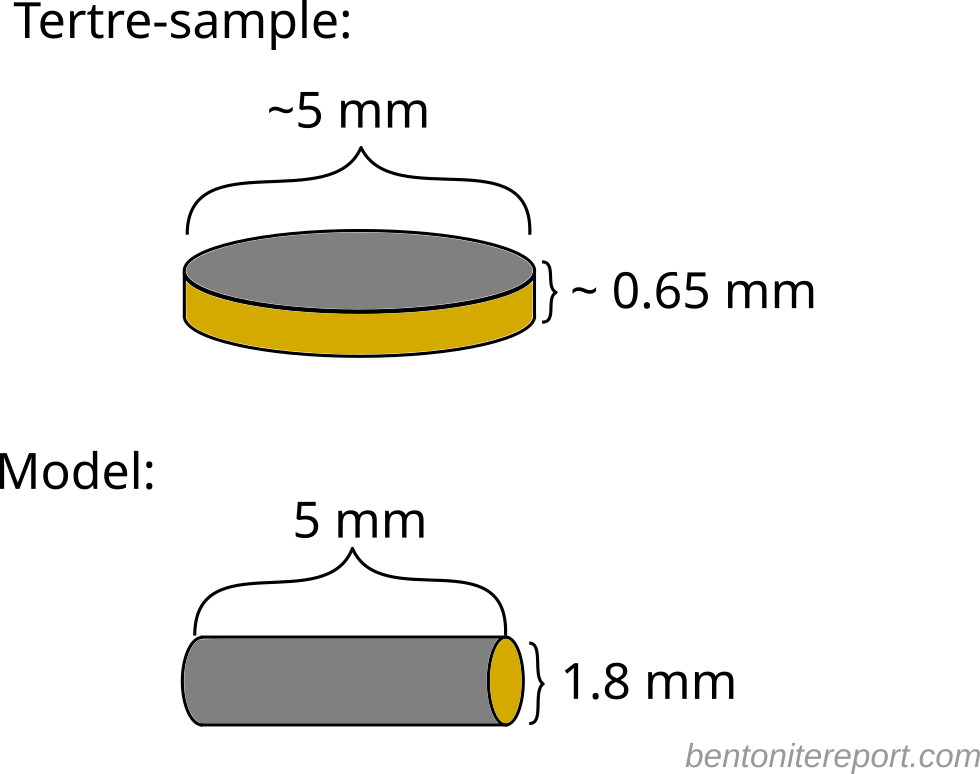
We choose the “equivalent” samples to have the same volume as the Tertre-samples, and set the length of the “equivalent” samples equal to the diameter of the Tertre-samples. As a consequence, the interface area to the external solution (indicated in yellow in the above figure) in the “equivalent” sample is half the value of the Tertre-sample, which obviously will influence the detailed diffusional behavior. There will also be a difference in diffusional behavior because the “equivalent” sample has a larger part of the exchangeable ions positioned further from the interface. But we expect similar equilibrium states in the model, as we choose the total external reservoir volume to be the same as in the Tertre-tests (note that the model has an external reservoir on each side of the sample, while the Tertre-tests have a single external reservoir). The geometrical model parameters are listed in the table below.
| Clay density | 1.8 g/cm3 |
| Clay porosity | 0.357 |
| \(c_\mathrm{IL}\) (CEC) | 9.0 M (1.79 eq/kg) |
| Cross section area | 2.5 mm2 |
| Reservoir volumes | 75 ml + 75 ml |
Although the model does not reproduce the exact conditions of the Tertre-tests, we can use it to explore several principal features in such tests. In particular, we can explore the ion exchange equilibrium, the effect of possible interface transfer resistance, and the effect of electromigration (i.e. induced electric potential differences due to differences in mobility of the involved ions). Note that the cation exchange capacity for vermiculite is considerably larger than for bentonite. The high cation exchange capacity and density result in a very large value (9.0 M) for \(c_\mathrm{IL}\) — the central parameter involved in Donnan equilibrium calculations in the homogeneous mixture model.
As mentioned, the initial conditions are a pure Ca-clay (i.e. only calcium ions present, which compensate vermiculite structural charge), and pure NaCl solutions of various concentrations in the reservoirs. Clearly, such conditions will initiate an exchange process, where calcium migrates out into the reservoirs and sodium migrates into the clay, until these components are in equilibrium.
We present the modeling in stages, in order to observe the influence of the various mechanisms as clearly as possible. First we explore a model without interface transfer resistance and without influence from electromigration. Then we add electromigration (by giving different diffusivity to different ions), and finally we also add interface transfer resistance.
The fate of chloride in systems like these will be explored in a separate prediction, presented at the end of the blog post.
No interface transfer resistance, no electromigration
As our first case, we look at how the Na-for-Ca exchange process proceeds without any interface transfer resistance and without electromigration. In the model, this means that Donnan equilibrium is maintained directly at the interfaces between clay and external reservoirs. We also chose the diffusivity of all involved ions (Na, Ca, Cl) to be the same, thus eliminating any electromigration effects. Generally in this modeling exercise we will choose the individual diffusivities for calcium and sodium as 0.8⋅10-11 m2/s, and 1.33⋅10-11 m2/s, respectively. These correspond to values reported in Tertre et al. (2015), obtained from molecular dynamics simulations (although the sodium self-diffusivity is reported to vary between approximately 4⋅10-11 m2/s and 1⋅10-11 m2/s). In this first case, however, where all species should have the same diffusivity, we chose all ions to have the individual diffusivity for sodium.
| \(D_\mathrm{Na}^\mathrm{clay}\) | 1.33⋅10-11 m2/s |
| \(D_\mathrm{Ca}^\mathrm{clay}\) | 1.33⋅10-11 m2/s |
| \(D_\mathrm{Cl}^\mathrm{clay}\) | 1.33⋅10-11 m2/s |
This choice means that we may overestimate the outflux rate in the present model, as the calcium diffusivity is chosen “too large”. On the other hand, as we are modeling an exchange process, choosing a smaller sodium diffusivity may underestimate the outflux rate. This is the compromise that always has to be made, if we don’t want to invoke the Nernst-Planck framework. (In the next modeling case, where we include electromigration, this choice for the diffusivities will be further discussed.)
Below is shown the amount Ca diffused out as a function of time for various external NaCl concentrations (1.0 M to 0.003 M)
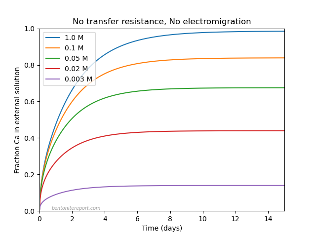
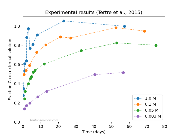
We have also included the experimental results from Tertre et al. (2015), for a direct comparison. The outflux is presented in these diagrams in terms of the fraction of the initial amount of calcium that has diffused out as a function of time. The amount calcium diffused out in the models is seen to level off at different values, reflecting the established ion exchange equilibrium. We see the same principal behavior in the experimental results. The exact values of the equilibrium concentrations are not the same in the experiment and model, indicating a difference between the selectivity coefficient in the model and in the experiment. As discussed in Birgersson (2017), the Ca/Na selectivity coefficient (\(K\)) in the homogeneous mixture model relates to activity coefficients as
\begin{equation} K \approx 2 \frac{\left (\gamma^\mathrm{int}_\mathrm{Na} \right )^2} {\gamma^\mathrm{int}_\mathrm{Ca}} \cdot c_\mathrm{IL} \tag{1} \end{equation}
where \(\gamma^\mathrm{int}_\mathrm{Na}\) and \(\gamma^\mathrm{int}_\mathrm{Ca}\) are the activity coefficients for sodium and calcium, respectively, in the interlayer domain. The way we implement the current model is equivalent to setting these parameters equal to unity (at the moment, the numerical tool does not handle activity coefficients).
Comparing model and experiments, it appears as if more calcium is expelled for a given external concentration in the tests (especially at the lower concentrations). This may indicate that the interlayer activity coefficient for calcium is larger than the square of the sodium activity coefficient in this particular system. However, we note that the selectivity coefficient also depend on \(c_\mathrm{IL}\) (eq. 1), which at these extreme conditions (high CEC, high density) is very sensitive to the actual value of the density. The difference between model and experiments could thus also be due to a difference in adopted density.
We note that the time to reach equilibrium is very different in the model as compared with the experiments. Although the model set-up is not fully equivalent to the experimental conditions, we expect similar time scales, as the geometry and diffusion parameters are chosen to be similar. The much longer time it takes for the experimental samples to equilibrate — especially those performed with lower initial NaCl concentration — must therefore be associated with a mechanism not included in the present model.
Looking at the modeled oufluxes in a bit more detail, we also note that the time to reach equilibrium increases with increasing NaCl concentration (opposite to the experimental behavior). Naively, one could think that this behavior is because more calcium must diffuse out for larger initial NaCl concentrations. But, for the simplest type of out-diffusion process, the time scale is actually independent of the absolute value of the amount of substance. The reason for the the observed delay at higher NaCl concentrations in the model is instead because the boundary conditions evolve differently in the different models, as calcium enters the reservoirs; for high initial NaCl concentration, the boundary concentration in the clay is essentially zero at all times, but for lower initial NaCl concentrations the boundary concentration instead continuously rises from zero to the equilibrium value. Therefore, the low NaCl concentration systems get an extra boost initially with an increased gradient (relatively speaking) and thus an increased outflux (relatively speaking).
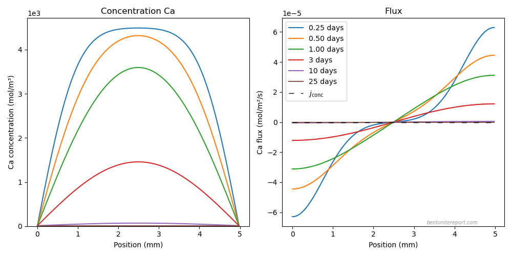
Here are snapshots of the internal calcium concentration and flux for initial NaCl concentration 1.0 M1
And here are the same quantities for the 0.05 M case
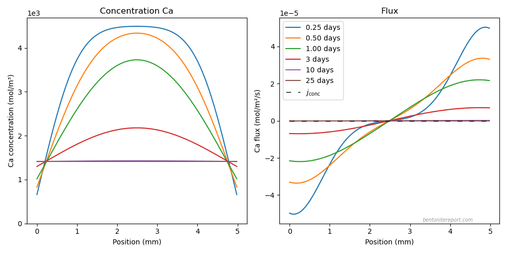
Note how the boundary concentrations reach the equilibrium value from below in this latter case.
Including electromigration
We include the effects of electromigration by assigning each ion its own diffusivity. In line with what Tertre et al. (2015) evaluate for calcium in molecular dynamics simulations, we now set the calcium diffusivity to 0.8⋅10-11 m2/s, while keeping the previous value for sodium. Moreover, the chloride diffusivity is set to give the same chloride/sodium diffusivity ratio as for bulk water. All adopted diffusivities are listed in the table below.
| \(D_\mathrm{Na}^\mathrm{clay}\) | 1.33⋅10-11 m2/s |
| \(D_\mathrm{Ca}^\mathrm{clay}\) | 0.8⋅10-11 m2/s |
| \(D_\mathrm{Cl}^\mathrm{clay}\) | 2.03⋅10-11 m2/s |
The results with electromigration active are quite interesting
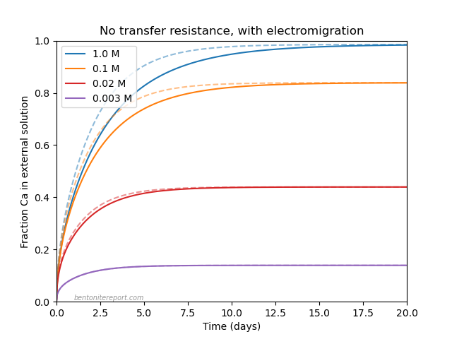
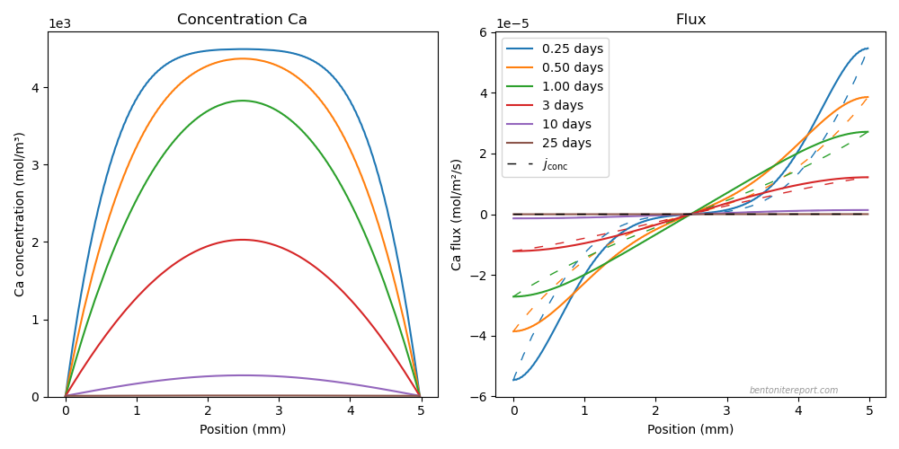
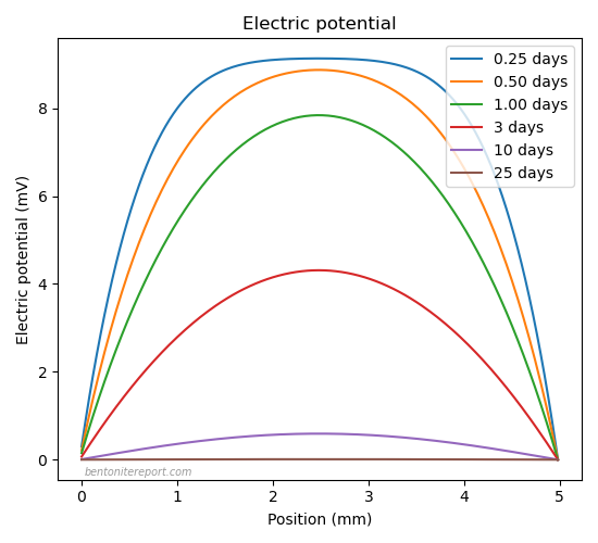
The results from the previous modeling — without electromigration and with a larger diffusion coefficient for calcium — are included in the left diagram as dashed lines. We note that the equilibration time increases for the systems with large external concentration, while equilibration takes essentially the same time as before for the lowest NaCl concentrations. We get more information about what is going on by looking at the evolutions for concentrations, electric potential and fluxes. Here are snapshots for the 1.0 M system
And here are the corresponding plots for the 0.003 M system
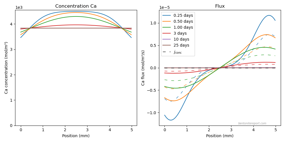
Note that the electric potential differences are quite profound in these systems. Initially in the 1.0 M system, the electric potential difference between the interface region and the middle of the sample is above 8 mV.2 Note that this substantial “diffusion potential” is not induced by choosing extreme values of the diffusivity ratios (as we have done earlier), but is a consequence of having two different types of cations with substantial concentrations in the system.
The electric potential differences appear on quite short distances, which implies large electric fields (the electric field is given by the gradient of the potential). What is going on physically is that the faster sodium is diffusing into the sample, inducing an electric field directed out of the sample. This electric field retards the sodium influx and enhances the calcium outflux. This electromigration effect is noted to be mostly active during the first few days of the process; after 3 days, the total diffusive flux in both systems is similar to the concentration gradient contribution (\(j_\mathrm{conc}\)), i.e. after this point the calcium flux is mainly “Fickian”.
The effect of the initial electromigration boost for calcium is that the process is essentially finished for the 0.003 M system; after this initial phase, this system is essentially in equilibrium with the external reservoir. Systems with larger external concentration, on the other hand, still have substantial amounts of calcium that should diffuse out, and this transport is not boosted as significantly by electromigration. As a consequence, the equilibration process as a whole takes longer time, the larger the external concentration. In fact, the progress of the 0.003 M system is essentially independent of the value of the calcium diffusivity (but depends on the sodium diffusivity, which has not changed). The high concentration systems, on the other hand, appear to initially “diffuse” with a rate set by the sodium diffusivity, but then becomes more and more controlled by the value of the calcium diffusivity.
The present analysis clearly demonstrates that the effect of electromigration in these systems is the opposite of what is claimed in Tournassat and Steefel (2015). As we have already discussed in the review of this publication, the alternative “interpretation” put forward there is completely untenable, where it appears as if the authors simply by hand has put in various values of the sodium diffusivity in order for the model to reproduce the experimental results. At the same time they clearly state that the effect — i.e an apparent decrease of the calcium diffusivity with decreasing external NaCl concentration — is supposed to be due to electromigration. As we can see here, from a model where electromigration evidently is included, this mechanism rather has the effect of increasing the apparent out-diffusion as the external NaCl concentration is decreased. Perhaps needless to say, I strongly suspect that no actual analysis of the electromigration was performed in this modeling exercise in Tournassat and Steefel (2015).
Including interface transfer resistance
We note that a model that includes electromigration, but still does not account for possible interface transfer resistance, generally predicts a too fast calcium outflux. This is especially true for the tests performed at low initial NaCl concentration: the 0.003 M system is seen to have reached equilibrium before day 5 in the model, while the experimental results suggest a process that lasts 50 days or more.
In the next stage of the modeling we add a filter component at the interfaces between clay and external solutions, to account for interface transfer resistance. Donnan equilibrium is now maintained at the interfaces between filters and clay. The Tertre-tests do not include filters as system components, but here we use filters to model a general transfer resistance, and to observe its consequences. The filter properties, together with adopted diffusion coefficients, are listed in the table below.
| Filter length | 0.4 mm |
| Filter porosity | 0.357 |
| \(D_\mathrm{Na}^\mathrm{filter}\) | 2.66⋅10-9 m2/s |
| \(D_\mathrm{Ca}^\mathrm{filter}\) | 1.6⋅10-9 m2/s |
| \(D_\mathrm{Cl}^\mathrm{filter}\) | 4.06⋅10-9 m2/s |
| \(D_\mathrm{Na}^\mathrm{clay}\) | 1.33⋅10-11 m2/s |
| \(D_\mathrm{Ca}^\mathrm{clay}\) | 0.8⋅10-11 m2/s |
| \(D_\mathrm{Cl}^\mathrm{clay}\) | 2.03⋅10-11 m2/s |
Note that the filter diffusivities are not aimed to have realistic values; the chosen filter diffusivities are larger than the corresponding bulk water diffusivities (they are set to be 200 times larger than the clay diffusivities). The filter components are there simply to add some transfer resistance (the total transport capacity for the filter is quantified by the combination of parameters \(\phi_\mathrm{filter}\cdot D_\mathrm{filter}/L_\mathrm{filter}\)). In the present case, the chosen filter parameter values contribute to a relatively large transport capacity.
The modeled results now look like this (and are also compared with the Tertre results)
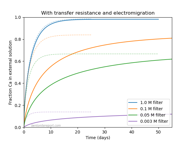
In the left diagram we have also indicated results from the previous model, which included electromigration but no interface transfer resistance (dashed lines).
We note that adding a constant finite interface transport capacity gives the correct principal model behavior as compared with experiment: the effect is large for low initial NaCl concentrations, while it is barely noticeable at the highest NaCl concentration (1.0 M). This is completely in line with how interface transfer resistance works, as we discussed in the context of cation tracer through-diffusion here. The principal explanation for the behavior is that the lower the “background concentration” is, the harder it is for the filter component (or the interface region, more generally) to supply the clay with all the cations that it requires, and to transport away the expelled ions. There is obviously a huge difference between the initial calcium concentration in the clay (4.5 M) and e.g. 0.025 M, or 0.0015 M.
Note that the filter parameters are here chosen in order to approximately match the outflux time scales observed experimentally. The effect is quite dramatic (compare e.g. the models at 0.1 M, with and without the filter component), yet the filter transport capacity is quite large. This illustrates the huge problem of handling divalent cations in a background of monovalent cations. We noted similar difficulties reported in strontium through-diffusion tests, which even used flushed filters in an effort to minimize transfer resistance.
The concentration profile and flux evolutions, for the 0.05 M model, look like this
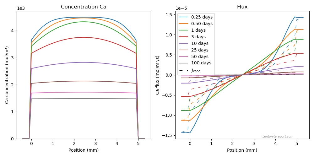
In the initial stages of the process, the concentration profile shows some significant curvature, but as time progresses, it becomes increasingly flat. In the prolonged later stage of the process, the profile is essentially completely flat, while the over-all concentration slowly falls with time. Flat non-equilibrium concentration profiles is a key signature of interface transfer resistance limiting the transport.
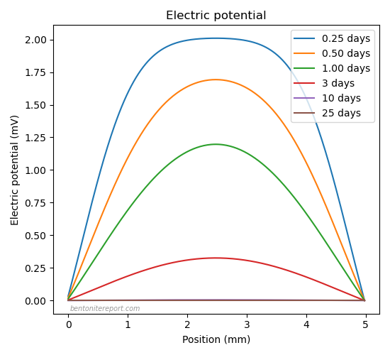
It is no surprise that the size of the developed electric potential is much smaller in a system limited by interface transfer resistance. Here is compared snapshots of the electric potential in the the 0.05 M system, with (left) and without (right) the filter component
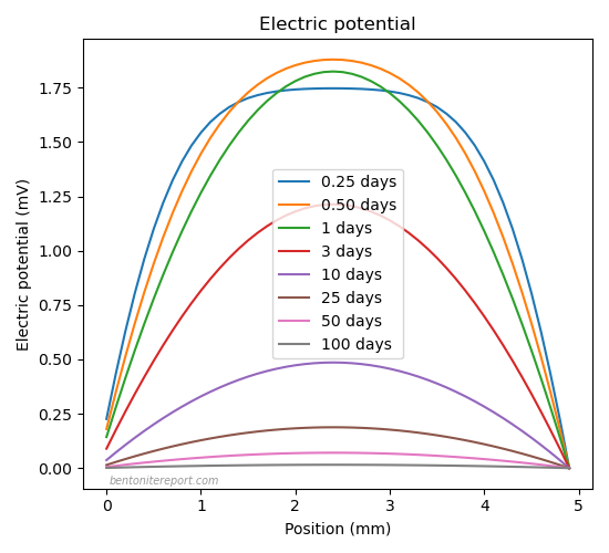
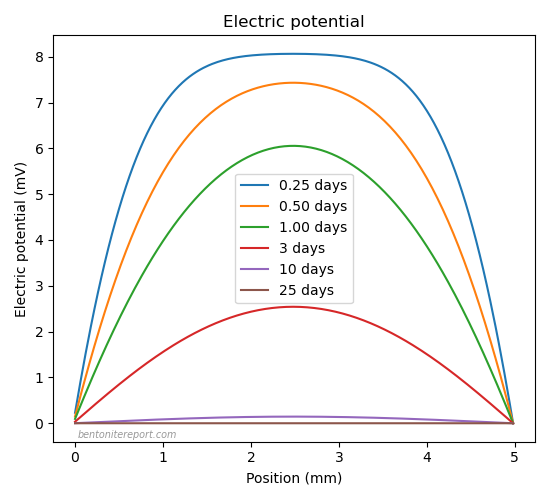
The maximum value of the electric potential lowers from about 8 mV without filters, to less than 2 mV with filters (the specific value depends, of course, on the chosen filter parameters).
The development of flat non-equilibrium concentration profiles is in complete contrast to the behavior of the system without interface transfer resistance. Here is a comparison between the concentration profile evolutions with (full lines) and without (dashed lines) filter, for the case of 0.05 M NaCl.
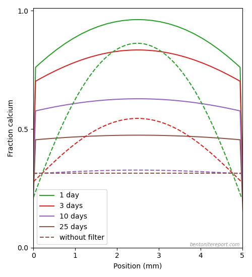
We can compare these distinctly different profile evolutions with experimental profile snapshot presented in Tertre et al. (2015).
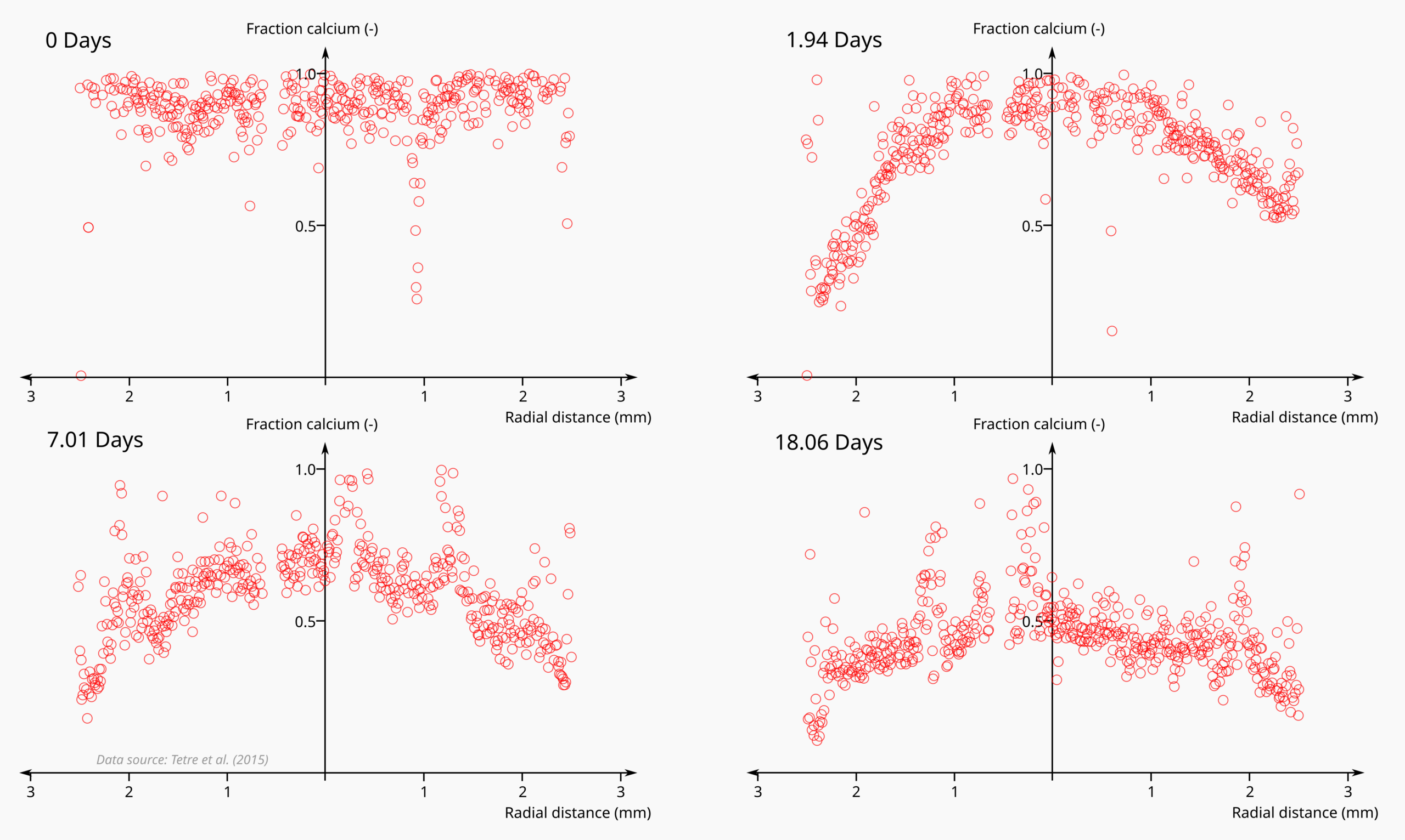
Here we should keep in mind that the Tertre-samples are not geometrically fully equivalent to the models. Yet, also the Tertre-tests reveal a curved concentration profile that progressively becomes flat — the signature behavior for a process limited by interface transfer resistance. Note that the latest snapshot presented in Tertre et al. (2015) (at 18.06 days) is still far from equilibrium; according to the outflux data in same study, the process lasts for about 50 days, and the equilibrium condition corresponds to about 20% of calcium in the clay.
The main conclusion from this analysis is that interface transfer resistance strongly influence the Na-for-Ca exchange process for lower NaCl concentrations in these types of tests. We can thus confirm the conclusion drawn in Tertre et al. (2015), while (again) dismissing the “reinterpretation” in Tournassat and Steefel (2015).
Chloride “pull-in”: a possible actual uphill diffusion effect
In the above analysis, we left out chloride from the discussion. With a huge \(c_\mathrm{IL}\) value, we expect the amount chloride entering the vermiculite to be very small in most of the Tertre-tests. But in principle, with an induced significant electric field directed out of the clay — caused by calcium diffusivity being substantially lower than sodium diffusivity — it is clear that a negatively charged ion will be pulled in. At least in regular bentonite samples, this effect may actually result in real uphill diffusion,3 which perhaps even can be detected experimentally.
For this model, we change the parameters to correspond to a “normal” montmorillonite sample, with substantial cross sectional area and length, in order to be relatively easily sectioned and analyzed.4
| Sample length | 10 mm |
| Sample density | 1.6 g/cm3 |
| Sample porosity | 0.429 |
| \(c_\mathrm{IL}\) (CEC) | 3.17 M (0.85 eq/kg) |
| Cross section area | 3.14 cm2 |
| Reservoir volumes | 250 ml + 250 ml |
| \(D_\mathrm{Na}^\mathrm{clay}\) | 2.8⋅10-11 m2/s |
| \(D_\mathrm{Ca}^\mathrm{clay}\) | 0.8⋅10-11 m2/s |
| \(D_\mathrm{Cl}^\mathrm{clay}\) | 3.4⋅10-11 m2/s |
Here we have chosen diffusivities to roughly correspond to what has been measured by Kozaki et al. (2000;2001;2005) in montmorillonite5 at the chosen density.
As in the previous models, we choose the clay to initially contain only calcium ions, and we choose the external reservoirs to initially contain pure 1.0 M NaCl solutions. With this external concentration, we expect negligible filter transfer resistance (filters are therefore not included) and we are assured that a substantial amount of chloride actually enters the clay.
Similar to the modeled Tertre-tests, the difference in mobility between calcium and sodium induces an electric field directed out of the clay sample. The evolution of the electric potential in this model looks like this
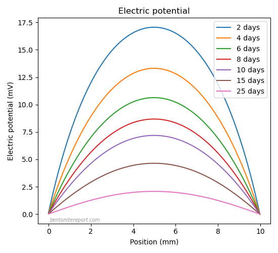
Note the quite large electric potential difference in the initial stages of the exchange process, with a maximum electric potential of about 20 mV. The corresponding concentration and flux evolutions for chloride look like this
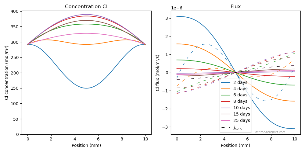
The flux diagram provides a quantitative picture of the uphill migration: up until about day 10, the total chloride flux (full lines) is directed opposite to the flux contribution from the concentration gradient (dashed lines), in the whole clay domain or in parts of it. In this time interval, where electromigration dominates, the chloride quite quickly forms a “bump” in the clay with concentrations that are larger than the corresponding equilibrium concentration (which is set at the reservoir interfaces). In later stages of the process, this “bump” diffuses out relatively slowly, as the transport now has a more “Fickian” character (the out-diffusion is actually even slightly retarded by the remaining electric field). It could consequently be possible to detect such a “bump” experimentally. The effect could be made more pronounced if calcium is replaced by an even slower ion, e.g. strontium or barium (with even larger electric potentials).
Footnotes
[1] The flux diagrams show both the total flux and the flux contribution from the concentration gradient. In this case, with no active electromigration mechanisms, these two fluxes coincide, and the concentration gradient contribution does not show (it is plotted with the same color as the total flux, but with dashed lines). Definitions of the various fluxes is found here.
[2] In all electric potential diagrams presented in this blog post, we choose the reference potential as zero in the clay at the interfaces to the external solutions. There is of course an additional Donnan potential step across the interface, which is different for different external NaCl concentrations. We don’t focus on the Donnan potentials here, but with the chosen reference, the reservoirs are at various positive potentials.
[3] It is important to distinguish a real uphill effect from the seeming uphill effect, which we have discussed massively on the blog. The seeming uphill effect is not caused by electromigration, and is observed in steady-state. A real uphill effect, in contrast, is an effect of electromigration, and is not maintained in steady-state.
[4] Analyzing ions in a bentonite sample is of course always burdened with difficulties. We have e.g. discussed the issue of interface excess here.
[5] Note that the Kozaki data is mainly for pure Na-montmorillonite, while the initial state of the model is pure Ca-montmorillonite.