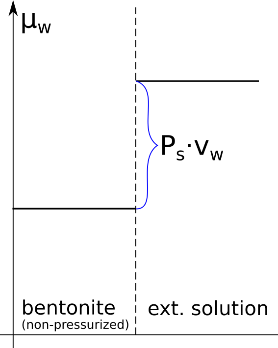
A testable difference
In the homogeneous mixture model, the effective diffusion coefficient for an ion in bentonite is evaluated as
\begin{equation} D_e = \phi \cdot \Xi \cdot D_c \tag{1} \end{equation}
where \(\phi\) is the porosity of the sample, \(D_c\) is the macroscopic pore diffusivity of the presumed interlayer domain, and \(\Xi\) is the ion equilibrium coefficient. \(\Xi\) quantifies the ratio between internal and external concentrations of the ion under consideration, when the two compartments are in equilibrium.
In the effective porosity model, \(D_e\) is instead defined as
\begin{equation} D_e = \epsilon_\mathrm{eff}\cdot D_p \tag{2} \end{equation}
where \(\epsilon_\mathrm{eff}\) is the porosity of a presumed bulk water domain where anions are assumed to reside exclusively, and \(D_p\) is the corresponding pore diffusivity of this bulk water domain.
We have discussed earlier how the homogeneous mixture and the effective porosity models can be equally well fitted to a specific set of anion through-diffusion data. The parameter “translation” is simply \(\phi\cdot \Xi \leftrightarrow \epsilon_\mathrm{eff}\) and \(D_c \leftrightarrow D_p\). It may appear from this equivalency that diffusion data alone cannot be used to discriminate between the two models.
But note that the interpretation of how \(D_e\) varies with background concentration is very different in the two models.
- In the homogeneous mixture model, \(D_c\) is not expected to vary with background concentration to any greater extent, because the diffusing domain remains essentially the same. \(D_e\) varies in this model primarily because \(\Xi\) varies with background concentration, as a consequence of an altered Donnan potential.
- In the effective porosity model, \(D_p\) is expected to vary, because the volume of the bulk water domain, and hence the entire domain configuration (the “microstructure”), is postulated to vary with background concentration. \(D_e\) thus varies in this model both because \(D_p\) and \(\epsilon_\mathrm{eff}\) varies.
A simple way of taking into account a varying domain configuration (as in the effective porosity model) is to assume that \(D_p\) is proportional to \(\epsilon_\mathrm{eff}\) raised to some power \(n – 1\), where \(n > 1\). Eq. 2 can then be written
\begin{equation} D_e = \epsilon_\mathrm{eff}^n\cdot D_0 \tag{3} \end{equation} \begin{equation}\text{ (effective porosity model)} \end{equation}
where \(D_0\) is the tracer diffusivity in pure bulk water. Eq. 3 is in the bentonite literature often referred to as “Archie’s law”, in analogy with a similar evaluation in more conventional porous systems. Note that with \(D_0\) appearing in eq. 3, this expression has the correct asymptotic behavior: in the limit of unit porosity, the effective diffusivity reduces to that of a pure bulk water domain.
Eq. 3 shows that \(D_e\) in the effective porosity model is expected to depend non-linearly on background concentration for constant sample density. In contrast, since \(D_c\) is not expected to vary significantly with background concentration, we expect a linear dependence of \(D_e\) in the homogeneous mixture model. Keeping in mind the parameter “translation” \(\phi\cdot\Xi \leftrightarrow \epsilon_\mathrm{eff}\), the prediction of the homogeneous mixture model (eq. 1) can be expressed1
\begin{equation} D_e = \epsilon_\mathrm{eff}\cdot D_c \tag{4} \end{equation} \begin{equation} \text{ (homogeneous mixture model)} \end{equation}
We have thus managed to establish a testable difference between the effective porosity and the homogeneous mixture model (eqs. 3 and 4). This is is great! Making this comparison gives us a chance to increase our process understanding.
Comparison with experiment
Van Loon et al. (2007)
It turns out that the chloride diffusion measurements performed by Van Loon et al. (2007) are accurate enough to resolve whether \(D_e\) depends on “\(\epsilon_\mathrm{eff}\)” according to eqs. 3 or 4. As will be seen below, this data shows that \(D_e\) varies in accordance with the homogeneous mixture model (eq. 4). But, since Van Loon et al. (2007) themselves conclude that \(D_e\) obeys Archie’s law, and hence complies with the effective porosity model, it may be appropriate to begin with some background information.
Van Loon et al. (2007) report three different series of diffusion tests, performed on bentonite samples of density 1300, 1600, and 1900 kg/m3, respectively. For each density, tests were performed at five different NaCl background concentrations: 0.01 M, 0.05 M, 0.1 M, 0.4 M, and 1.0 M. The tests were evaluated by fitting the effective porosity model, giving the effective diffusion coefficient \(D_e\) and corresponding “effective porosity” \(\epsilon_\mathrm{eff}\) (it is worth repeating that the latter parameter equally well can be interpreted in terms of an ion equilibrium coefficient).
Van Loon et al. (2007) conclude that their data complies with eq. 3, with \(n = 1.9\), and provide a figure very similar to this one

Here are compared evaluated values of effective diffusivity and “effective porosity” in various tests. The test series conducted by Van Loon et al. (2007) themselves are labeled with the corresponding sample density, and the literature data is from García-Gutiérrez et al. (2006)2 (“Garcia 2006”) and the PhD thesis of A. Muurinen (“Muurinen 1994”). Also plotted is Archie’s law with \(n\) =1.9. The resemblance between data and model may seem convincing, but let’s take a further look.
Rather than lumping together a whole bunch of data sets, let’s focus on the three test series from Van Loon et al. (2007) themselves, as these have been conducted with constant density, while only varying background concentration. This data is thus ideal for the comparison we are interested in (we’ll get back to commenting on the other studies).
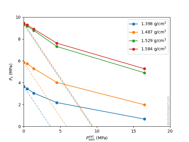
It may also be noted that the published plot contains more data points (for these specific test series) than are reported in the rest of the article. Let’s therefore instead plot only the tabulated data.3 The result looks like this

Here we have also added the predictions from the homogeneous mixture model (eq. 4), where \(D_c\) has been fitted to each series of constant density.
The impression of this plot is quite different from the previous one: it should be clear that the data of Van Loon et al. (2007) agrees fairly well with the homogeneous mixture model, rather than obeying Archie’s law. Consequently, in contrast to what is stated in it, this study refutes the effective porosity model.
The way the data is plotted in the article is reminiscent of Simpson’s paradox: mixing different types of dependencies of \(D_e\) gives the illusion of a model dependence that really isn’t there. Reasonably, this incorrect inference is reinforced by using a log-log diagram (I have warned about log-log plots earlier). With linear axes, the plots give the following impression

This and the previous figure show that \(D_e\) depends approximately linearly on “\(\epsilon_\mathrm{eff}\)”, with a slope dependent on sample density. With this insight, we may go back and comment on the other data points in the original diagram.
García-Gutiérrez et al. (2006) and Muurinen et al. (1988)
The tests by García-Gutiérrez et al. (2006) don’t vary the background concentration (it is not fully clear what the background concentration even is4), and each data point corresponds to a different density. This data therefore does not provide a test for discriminating between the models here discussed.
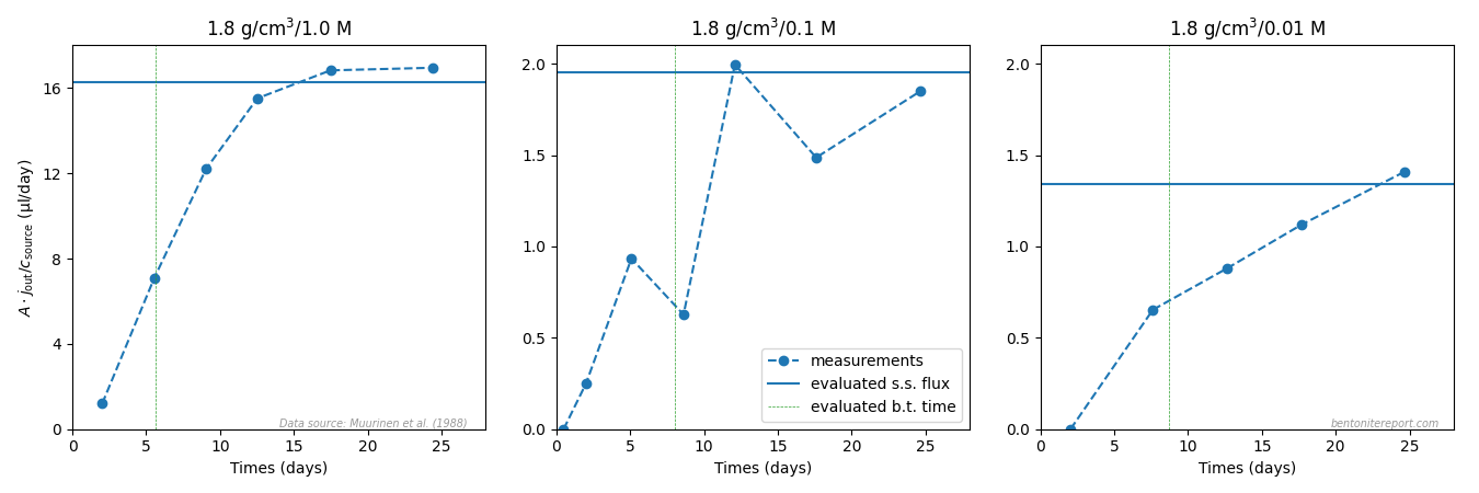
I have had no access to Muurinen (1994), but by examining the data, it is clear that it originates from Muurinen et al. (1988), which was assessed in detail in a previous blog post. This study provides two estimations of “\(\epsilon_\mathrm{eff}\)”, based on either breakthrough time or on the actual measurement of the final state concentration profile. In the above figure is plotted the average of these two estimations.5
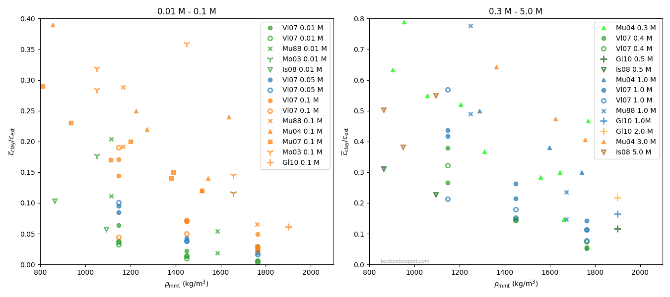
One of the test series in Muurinen et al. (1988) considers variation of density while keeping background concentration fixed, and does not provide a test for the models here discussed. The data for the other two test series is re-plotted here, with linear axis scales, and with both estimations for “\(\epsilon_\mathrm{eff}\)”, rather than the average6

As discussed in the assessment of this study, I judge this data to be too uncertain to provide any qualitative support for hypothesis testing. I think this plot confirms this judgment.
Glaus et al. (2010)
The measurements by Van Loon et al. (2007) are enough to convince me that the dependence of \(D_e\) for chloride on background concentration is further evidence for that a homogeneous view of compacted bentonite is principally correct. However, after the publication of this study, the same authors (partly) published more data on chloride equilibrium, in pure Na-montmorillonite and “Na-illite”,7 in Glaus et al. (2010).
This data certainly shows a non-linear relation between \(D_e\) and “\(\epsilon_\mathrm{eff}\)” for Na-montmorillonite, and Glaus et al. (2010) continue with an interpretation using “Archie’s law”. Here I write “Archie’s law” with quotation marks, because they managed to fit the expression to data only by also varying the prefactor. The expression called “Archie’s law” in Glaus et al. (2010) is
\begin{equation} D_e = A\cdot\epsilon_\mathrm{eff}^n \tag{5} \end{equation}
where \(A\) is now a fitting parameter. With \(A\) deviating from \(D_0\), this expression no longer has the correct asymptotic behavior as expected when interpreting \(\epsilon_\mathrm{eff}\) as quantifying a bulk water domain (see eq. 3). Nevertheless, Glaus et al. (2010) fit this expression to their measurements, and the results look like this (with linear axes)

Here is also plotted the prediction of the homogeneous mixture model (eq. 4). For the montmorillonite data, the dependence is clearly non-linear, while for the “Na-illite” I would say that the jury is still out.
Although the data for montmorillonite in Glaus et al. (2010) is non-linear, there are several strong arguments for why this is not an indication that the effective porosity model is correct:
- Remember that this result is not a confirmation of the measurements in Van Loon et al. (2007). As demonstrated above, those measurements complies with the homogeneous mixture model. But even if accepting the conclusion made in that publication (that Archie’s law is valid), the Glaus et al. (2010) results do not obey Archie’s law (but “Archie’s law”).
- The four data points correspond to background concentrations of 0.1 M, 0.5 M, 1.0 M, and 2.0 M. If “\(\epsilon_\mathrm{eff}\)” represented the volume of a bulk water phase, it is expected that this value should level off, e.g. as the Debye screening length becomes small (Van Loon et al. (2007) argue for this). Here “\(\epsilon_\mathrm{eff}\)” is seen to grow significantly, also in the transition between 1.0 M and 2.0 M background concentration.
- These are Na-montmorillonite samples of dry density 1.9 g/cm3. With an “effective porosity” of 0.067 (the 2.0 M value), we have to accept more than 20% “free water” in these very dense systems! This is not even accepted by other proponents of bulk water in compacted bentonite.
Furthermore, these tests were performed with a background of \(\mathrm{NaClO_4}\), in contrast to Van Loon et al. (2007), who used chloride also for the background. The only chloride around is thus at trace level, and I put my bet on that the observed non-linearity stems from sorption of chloride on some system component.
Insight from closed-cell tests
Note that the issue whether or not \(D_e\) varies linearly with “\(\epsilon_\mathrm{eff}\)” at constant sample density is equivalent to whether or not \(D_p\) (or \(D_c\)) depends on background concentration. This is similar to how presumed concentration dependencies of the pore diffusivity for simple cations (“apparent” diffusivities) have been used to argue for multi-porosity in compacted bentonite. For cations, a closer look shows that no such dependency is found in the literature. For anions, it is a bit frustrating that the literature data is not accurate or relevant enough to fully settle this issue (the data of Van Loon et al. (2007) is, in my opinion, the best available).
However, to discard the conceptual view underlying the effective porosity model, we can simply use results from closed-cell diffusion studies. In Na-montmorillonite equilibrated with deionized water, Kozaki et al. (1998) measured a chloride diffusivity of \(1.8\cdot 10^{-11}\) m2/s at dry density 1.8 g/cm3.8 If the effective porosity hypothesis was true, we’d expect a minimal value for the diffusion coefficient9 in this system, since \(\epsilon_\mathrm{eff}\) approaches zero in the limit of vanishing ionic strength. Instead, this value is comparable to what we can evaluate from e.g. Glaus et al. (2010) at 1.9 cm3/g, and 2.0 M background electrolyte: \(D_e/\epsilon_\mathrm{eff} = 7.2\cdot 10^{-13}/0.067\) m2/s = \(1.1\cdot 10^{-11}\) m2/s.
That chloride diffuses just fine in dense montmorillonite equilibrated with pure water is really the only argument needed to debunk the effective porosity hypothesis.
Footnotes
[1] Note that \(\epsilon_\mathrm{eff}\) is not a parameter in the homogeneous mixture model, so eq. 4 looks a bit odd. But it expresses \(D_e\) if \(\phi\cdot \Xi\) is interpreted as an effective porosity.
[2] This paper appears to not have a digital object identifier, nor have I been able to find it in any online database. The reference is, however, Journal of Iberian Geology 32 (2006) 37 — 53.
[3] This choice is not critical for the conclusions made in this blog post, but it seems appropriate to only include the data points that are fully described and reported in the article.
[4] García-Gutiérrez et al. (2004) (which is the study compiled in García-Gutiérrez et al. (2006)) state that the samples were saturated with deionized water, and that the electric conductivity in the external solution were in the range 1 — 3 mS/cm.
[5] The data point labeled with a “?” seems to have been obtained by making this average on the numbers 0.5 and 0.08, rather than the correctly reported values 0.05 and 0.08 (for the test at nominal density 1.8 g/cm3 and background concentration 1.0 M).
[6] Admittedly, also the data we have plotted from the original tests in Van Loon et al. (2007) represents averages of several estimations of “\(\epsilon_\mathrm{eff}\)”. We will get back to the quality of this data in a future blog post when assessing this study in detail, but it is quite clear that the estimation based on the direct measurement of stable chloride is the more robust (it is independent of transport aspects). Using these values for “\(\epsilon_\mathrm{eff}\)”, the corresponding plot looks like this

Update (220721): Van Loon et al. (2007) is assessed in detail here.
[7] To my mind, it is a misnomer to describe something as illite in sodium form. Although “illite” seems to be a bit vaguely defined, it is clear that it is supposed to only contain potassium as counter-ion (and that these ions are non-exchangeable; the basal spacing is \(\sim\)10 Å independent of water conditions). The material used in Glaus et al. (2010) (and several other studies) has a stated cation exchange capacity of 0.22 eq/kg, which in a sense is comparable to the montmorillonite material (a factor 1/4). Shouldn’t it be more appropriate to call this material e.g. “mixed-layer”?
[8] This value is the average from two tests performed at 25 °C. The data from this study is better compiled in Kozaki et al. (2001).
[9] Here we refer of course to the empirically defined diffusion coefficient, which I have named \(D_\mathrm{macr.}\) in earlier posts. This quantity is model independent, but it is clear that it should be be associated with the pore diffusivities in the two models here discussed (i.e. with \(D_c\) in the homogeneous mixture model, and with \(D_p\) in the effective porosity model).