Category Archives: Sorption

Assessment of chloride equilibrium concentrations: Glaus et al. (2010)

In the ongoing assessment of chloride equilibrium concentrations in bentonite, we here take a closer look at the study by Glaus et al. (2010), in the following referred to as Gl10. We thus assess the 4 points indicated here

Reading Gl10 gives the impression that the study consists solely of through-diffusion tests of a set of different tracers (HTO, sodium, chloride), in a set of different materials (Kaolinite, “Na-Illite”, Na-montmorillonite), at nominal density 1.9 g/cm³. A lot of additional information, however, is published in a later, completely separate publication: Glaus et al. (2011), which we will refer to as Gl11. Needless to say, this is a quite peculiar way of reporting a study. For instance, Gl10 do not provide any geometrical information about the samples (!), but this is found in Gl11; Gl11 also report corresponding out-diffusion measurements that apparently were made.¹

Even with the combined sources of Gl10 and Gl11, information is not entirely complete. For example, tests have been carried out in duplicates, but evaluated diffusion parameters are only reported as averages (table 2 in Gl10). Furthermore, the sources give contradictory information in some instances (this is further discussed below). Scraping both sources for information, these are the tests that have been performed, as far as I understand:

Through-diffusion

In total 8 separate tests were performed, with NaClO₄ background concentrations of 0.1 M, 0.5 M, 1.0 M and 2.0 M. These were performed in sequence in four different tests cells. Thus, two tests at 1.0 M background concentration were first performed in two different samples; thereafter, the same two samples were used for two additional tests at 2.0 M. Similarly, in two other samples, two 0.5 M tests were followed by two 0.1 M tests. The steady-state concentration profile in the clay was measured in one single test, performed at 0.1 M background concentration.
In this assessment we will also make use of the results from through-diffusion of water (HTO). These were made at background concentrations 0.1 M and 1.0 M. We will return to the question of whether they were carried out in the same samples as used for the chloride-diffusion experiments.
Out-diffusion

Most of the through-diffusion tests were followed by out-diffusion tests: after steady-state was reached, the external reservoirs were exchanged for tracer free solutions, and diffusion of chloride out of the sample was recorded.
Out-diffusion was tested on all samples at background concentrations 0.5 M and 2.0 M, and on one sample at background concentration 0.1 M.
Sorption

The montmorillonite material was tested for sorption of chloride, in suspensions with background concentrations of either perchlorate or chloride (at 0.5 M).
Equilibrium tests

At least one test was conducted to investigate the amount of ClO₄ in the clay after the sample was equilibrated with a specified external concentration.
Investigation of swelling during dismantling.

The samples were cylindrical with diameter 2.54 cm, and with slightly different lengths, close to 1.0 cm. The sample volume is thus roughly 5 cm³.

In the following, we mainly refer to the chloride diffusion tests in montmorillonite. Although the diffusion parameters are only reported as averages, each individual parameter is actually found in a single plot in Gl10 (“Fig. 6”). From this plot we can extract results from each individual through-diffusion test (see below).

In Gl10 are also presented breakthrough curves (flux vs. time) for four tests, one for each different background concentration. Similarly, in Gl11 are presented three flux-vs.-time plots for out-diffusion. As will be further discussed below, we have to do some combined guess- and detective work in order to identify these flux evolution curves with specific samples.

Material

The material is referred to as montmorillonite “from Milos”, and was prepared specifically for the study. Bentonite from Milos (Greece), purchased from Süd-Chemie (now Clariant), was repeatedly washed in strong NaCl solutions to remove most of the accessory minerals and to convert the clay to essentially pure sodium-form. Excess NaCl was subsequently removed from the clay by dialysis. Gl10 present analyses of the chemical composition of both the used materials, as well as of a further purified 0.5 \(\mu\)m fraction of the montmorillonite material. From these analyses it is concluded that the used montmorillonite still contains some silica accessory minerals (3 — 4%), as well as some carbonate (calcite). We may thus assume a montmorillonite content of around 95%.

Concerning the cation population, Gl10 assert that the detected calcium is “most probably” present as CaCO₃ rather than being part of the exchangeable cations. However, as the purification procedure used here is quite similar to that used in Muurinen et al. (2004) — that we have assessed earlier — we may expect some influence of calcium on the exchangeable cations. Muurinen et al. (2004) measured a Na/Ca-ratio of approximately 90/10 in their material, which also contained some carbonate (as well as sulfate). Here we assume that the used Na-montmorillonite is basically a pure sodium system, but should keep in mind that the presence of calcium may somewhat influence the results, especially since the different samples are exposed to very different external sodium concentrations.

Sample density

The nominal density for all samples appears to be 1.9 g/cm³, but actual sample densities are not reported (in Gl10, it is even hard to find information on nominal density). However, results of HTO diffusion in four test (at 0.1 M and 1.0 M background concentration) indicate a considerably lower density. Porosities inferred from the breakthrough curves for these tests range between approximately 0.35 — 0.42. As is further discussed below, we here choose a range for the porosity of 0.321 — 0.394. Assuming a grain density of \(\rho_s\) = 2.8 g/cm³, this corresponds to a density range of 1.9 g/cm³ — 1.7 g/cm³ (effective montmorillonite density 1.87 g/cm³ — 1.66 g/cm³).

Uncertainty of external solutions

We have no reason to doubt the validity of the solutions used, and will assume no uncertainty here.

Evaluations from the diffusion tests

The chloride diffusion data in Gl10 and Gl11 is essentially analyzed in terms of the effective porosity model, although the fitted parameters are the “effective diffusivity” (\(D_e\)) and the “rock capacity factor” (\(\alpha\)). But for chloride, Gl10 use \(\alpha\) and \(\epsilon_\mathrm{eff}\) (the “effective porosity”) interchangeably.² To avoid confusion, we will only use the notation \(\epsilon_\mathrm{eff}\).

As mentioned, Gl10 only tabulate the mean values of \(D_e\) and \(\epsilon_\mathrm{eff}\) for each background concentration, but we can extract each individual parameter graphically. The extracted \(D_e\) and \(\epsilon_\mathrm{eff}\) are listed here.³

\(C_\mathrm{bkg}\) M	\(\epsilon_\mathrm{eff}\) (Gl10 fig. 6)	\(D_e\) 10^-13 m²/s (Gl10 fig. 6)	\(D_p\) 10^-12 m²/s eq. 1	\(D_p\) 10^-12 m²/s from sim.	\(j_\mathrm{ss}\) 10^-13 mol/m²/s from sim.	\(c^\mathrm{source}\) mol/m³ eq. 2
0.1	0.017	0.68	4.0	3.9/3.4	1.51/1.67	0.021
0.1	0.021	0.75	3.6	4.3 (profile)	1.8 (in text)	0.024 (in text)
0.5	0.036	2.5	6.8	6.6	5.46	0.022
0.5	0.036	2.5	6.8	6.3	11.7	0.046
1.0	0.050	4.9	9.8	10	10.9	0.023
1.0	0.050	4.6	9.2
2.0	0.068	7.4	11	10.6/10.5	16.3/16.8	0.022
2.0	0.066	6.9	10

With a single exception, the averages are identical with what is listed in table 2 in Gl10, which confirms the accuracy of the extracted parameters (for 1.0 M background concentration, the average \(\epsilon_\mathrm{eff}\) is 0.050 rather than the tabulated value 0.051). In the above table are also listed the corresponding pore diffusivities, evaluated as

\begin{equation} D_p = \frac{D_e}{\epsilon_\mathrm{eff}}. \tag{1} \end{equation}

From the flux and profile data found in Gl10 and Gl11, we can also evaluate several pore diffusivites ourselves. Such values are presented in the fifth column in the above table, and corresponding steady-state fluxes are found in the sixth column. Below is compared various flux vs. time data with my own simulations.

Regarding the breakthrough curves, the test design is here much better than what we have encountered in earlier assessments; the transient stage is properly sampled rather than that the data mainly represents a sequence of steady-state measurements.⁴ This makes the inference of diffusion parameters quite easy and robust.

Comparing the through-diffusion and out-diffusion results we can conclude that the data presented in Gl10 and Gl11 for background concentration 0.1 M most probably is for the same sample. Although the fitted parameters differ somewhat, the text of Gl11 states a steady state flux of 1.8⋅10^-13 mol/s/m² for the other 0.1 M sample, which was subsequently sectioned. As the presented through-diffusion flux is considerably smaller we may conclude that this is the same sample for which out-diffusion subsequently was conducted.

For the 0.5 M data, we can instead conclude that the two data sets must stem from two different samples, as the steady-state fluxes differ by roughly a factor of 2. For the 2.0 M data, the fitted parameters are very similar for the two test phases, which may indicate that they were measured in the same sample. However, the parameters are also very similar for the other test. The same is true for 1.0 M data (for which no out-diffusion was performed).

From steady-state fluxes and reported values of \(D_e\), we can calculate the corresponding tracer concentration in the source reservoir as

\begin{equation} c^\mathrm{source} = \frac{j_\mathrm{ss}\cdot L}{D_e} \tag{2} \end{equation}

where \(L\) is sample length.⁵ Source tracer concentrations evaluated in this way are presented in the last column in the above table (source concentration is only reported for a single test, in Gl11).

Finally, we can also look at the presented tracer profile at termination, which was determined in a single case,⁶ for one of the 0.1 M tests.

We note — as does Gl11 — that the concentration profile shows quite extensive interface excess, a topic that we have discussed in a separate blog post. The main focus of Gl11 is actually a modeling treatment of these regions, but here we focus on the linear interior part of the profile.⁷ Fitting a line to this part (see figure) we extract a slope of -22.0 nmol/g/m. Gl11 do not report the corresponding density profile (that most certainly was measured), but using the nominal density (1.9 g/cm³), gives a corresponding clay concentration gradient of \(\nabla c_\mathrm{ss} = -0.0418\) mol/m⁴. Combining this value with the steady-state flux (1.8⋅10^-13 mol/m²/s; reported in the text in Gl11), we can independently evaluate the pore diffusivity

\begin{equation} D_p = -\frac {j_\mathrm{ss}}{\nabla c_\mathrm{ss}} = \frac{1.8\cdot 10^{-13}}{0.0418} \;\mathrm{m^2/s} = 4.3 \cdot 10^{-12} \;\mathrm{m^2/s} \end{equation}

This is in reasonable agreement with the value evaluated from \(D_e\) and \(\epsilon_\mathrm{eff}\).

In conclusion, even though crucial information is missing in Gl10, the re-evaluations made here, with help from information in Gl11, confirm the adequacy of the reported parameters \(D_e\) and \(\epsilon_\mathrm{eff}\). A perhaps single conspicuous detail is that the source concentration in one of the 0.5 M tests appears to have been about twice as large as for any of the other tests. There may, of course, be a reasonable explanation for this.

Evaluating chloride equilibrium concentrations

As noted in earlier assessments, the convenient quantity expressing the chloride equilibrium in through-diffusion tests is the ratio \(\bar{c}(0) / c^\mathrm{source}\), where \(\bar{c}(0)\) denotes the tracer concentration within the clay, at the interface to the source reservoir (for details, see here).

From the reported values of \(\epsilon_\mathrm{eff}\), the most straightforward way to evaluate the chloride equilibrium concentrations is

\begin{equation} \frac{\bar{c}(0)}{c^\mathrm{source}} = \frac{\epsilon_\mathrm{eff}}{\phi} \tag{3} \end{equation}

where \(\phi\) is the (physical) porosity. Gl10 (or Gl11) don’t provide information on actual measured densities, leaving us little choice but to use the nominal density in order to get a value for \(\phi\) in eq. 3. However, Gl10 also provide data for corresponding water (HTO) diffusion measurements. As mentioned above, these measurements indicate densities significantly lower than the nominal value. The (graphically extracted) values for \(D_e\) and \(\epsilon_\mathrm{eff}\) for HTO are

\(C_\mathrm{bkg}\) M	\(\epsilon_\mathrm{eff}\) (Gl10 fig. 6)	\(D_e\) m²/s (Gl10 fig. 6)	\(D_p\) m²/s eq. 1	\(\rho_d\) g/cm³
0.1	0.352	1.7e-11	4.8e-11	1.81
0.1	0.402	1.7e-11	4.1e-11	1.67
1.0	0.401	2.0e-11	5.0e-11	1.68
1.0	0.421	1.9e-11	4.5e-11	1.62

For water, the effective porosity parameter is really an estimate of the physical porosity, and we can thus use this value to calculate a corresponding density, which is presented in the last column in the table.

Gl10 state

The diffusion of the various radioactive tracers (HTO, ²²Na, ³⁶Cl) was measured in sequence, each new tracer run was started after the out-diffusion of the previous tracer had been completed.

which is hard to interpret in any other way than that the above HTO parameters have been evaluated in the same samples in which chloride diffusion was tested. However, the protocol presented in Gl11 does not include any HTO diffusion “measured in sequence” (see above for information on the test protocol). The two sources evidently contain some contradictory information.⁸ Under any circumstance, as water diffusivity is claimed to be measured in samples with the same nominal density, we must assume a quite substantial uncertainty of the actual sample densities. In evaluating the chloride equilibrium concentrations, we therefore choose a porosity interval between the nominal value and the average given from the water parameters: \(\phi\sim\) 0.321 — 0.394. The table below lists the corresponding intervals for the chloride equilibrium concentrations

\(C_\mathrm{bkg}\) M	\(\epsilon_\mathrm{eff}\) (Gl10 fig. 6)	\(\bar{c}(0)/c^\mathrm{source}\) eq. 3	\(\bar{c}(0)/c^\mathrm{source}\) outflux (eq. 4) / profile
0.1	0.017	0.043 — 0.053	0.053 — 0.065 (o)
0.1	0.021	0.053 — 0.065	0.051 — 0.070 (p)
0.5	0.036	0.091 — 0.112
0.5	0.036	0.091 — 0.112	0.107 — 0.131 (o)
1.0	0.050	0.127 — 0.156
1.0	0.050	0.127 — 0.156
2.0	0.068	0.173 — 0.212	0.170 — 0.213 (o)
2.0	0.066	0.169 — 0.206

From the out-diffusion tests we can also evaluate the equilibrium concentrations “independently”, by integrating the flux. As discussed in the assessment of Van Loon et al. (2007), this integral (multiplied by sample area) gives one third of the total amount of tracers present in the clay at the start of the out-diffusion phase (these quantities are labelled “Acc.” in the above diagrams). With an estimate of the tracer concentration in the source reservoir, the equilibrium chloride concentration can thus be evaluated as

\begin{equation} \frac{\bar{c}(0)}{c^\mathrm{source}} = \frac{6\cdot N_\mathrm{right}}{\phi \cdot V_\mathrm{sample} \cdot c^\mathrm{source}} \tag{4} \end{equation}

where \(N_\mathrm{right}\) denotes the final amount of tracers in the target reservoir. The corresponding chloride equilibrium concentrations are listed in the last column in the above table.

Finally, we also look at the 0.1 M test for which the steady-state tracer concentration profile was recorded. Extrapolating the linear part to the clay/source interface, gives a chloride content of 0.282 nmol/g, which corresponds to a clay concentration interval of 5.37⋅10^-4 — 4.80⋅10^-4 mol/m³, using the porosity interval defined above.⁹ Given the source concentration (0.024 mol/m³), these values corresponds to a chloride equilibrium concentration ratio in the range 0.051 — 0.071.

The different ways of estimating chloride equilibrium concentrations provide a quite consistent picture (see above table). Although the information has been difficult to extract, it may thus seem that, in the end, all is good and well. However, we should note that the evaluated pore diffusivities show a quite peculiar dependency on background concentration.

Such a dependency, which has not been observed in earlier assessed studies, directly influence the evaluated equilibrium concentrations. As the breakthrough curves are so well sampled in the present study, this result can hardly be attributed to uncertainty in the values of \(D_p\). While Gl10 don’t explicitly identify this behavior (they do not evaluate \(D_p\)), a main focus of the study is actually to account for it, by means of “Archie’s law”, i.e. by suggesting a non-linear functional relationship between \(D_e\) and \(\epsilon_\mathrm{eff}\). I am strongly critical of such a treatment, but will refrain from discussing it here, as the focus of this assessment is the data itself rather than its interpretation (we have discussed this issue in a previous blog post).

An obvious alternative interpretation of this behavior is that chloride adsorbs on some system component, in the sense of becoming immobilized (what I have earlier dubbed true sorption). Gl11 test this hypothesis by performing additional batch sorption tests on the montmorillonite, in background solutions of NaCl and NaClO₄ (0.5 M) at various pH. Although they cannot exclude a “\(R_d\)” value of the order of 10^-4 m³/kg, they ultimately conclude that chloride do not sorb to any significant extent in these systems (and continues with “explaining” the behavior as resulting from other mechanisms).

I mean, however, that some experimental observations suggest that a sorption mechanism may be active. In addition to the above limit for the \(“R_d”\) value, we may note significant chloride sorption in the kaolinite samples, which were also studied in Gl10. There may of course be a reasonable explanation for why chloride sorption is observed in kaolinite, while it is not active in montmorillonite, but this issue is not really discussed in Gl10. Also, the recorded steady-state chloride content profile suggests a non-zero value at the interface to the target reservoir. This could, reasonably, indicate that some chloride is immobilized.

Perchlorate equilibrum concentrations

On the other hand, an additional argument against chloride sorption is that equilibrium perchlorate concentrations seem to be comparable with those evaluated for chloride. Gl11 don’t report perchlorate content directly, and we have to do some work to extract the corresponding equilibrium concentration in the 0.1 M sample that was sectioned. Gl11 plot the chloride tracer content for this sample together with “the concentration in the anion-accessible volume”, labelled \(c_\mathrm{acc}\).

\(c_\mathrm{acc}\) is, unsurprisingly, not a directly measured chloride concentration, but a quite elaborate interpretation of the data. From the unreported ClO₄ content, an “anion-accessible porosity” variable has been calculated, by simply multiplying the physical porosity by the ratio between internal and external ClO₄ concentrations. \(c_\mathrm{acc}\) is, in turn, defined as the actual measured chloride content distributed in a volume that corresponds to this “anion-accessible porosity”. By combining the reported chloride content (let’s call it \(\bar{n}_\mathrm{Cl}\)) and \(c_\mathrm{acc}\), we can thus de-derive the perchlorate equilibrium concentration as

\begin{equation} \frac{\bar{c}_\mathrm{ClO_4}}{0.1 \;\mathrm{M}} = \frac{\bar{n}_\mathrm{Cl}\cdot\rho}{c_\mathrm{acc}\cdot \phi} \end{equation}

Using this formula for the inner “linear” part of the profile (2 — 8 mm) gives the values 0.060, 0.059, 0.061 and 0.062, assuming nominal density. For porosity 0.394 the corresponding values are 0.044, 0.043, 0.044, and 0.045. We note that a range 0.043 — 0.062 for the equilibrium concentration ratio at 0.1 M background is in line with the previous evaluations. It should be noted, though, that this evaluation is for perchlorate, which not necessarily has the same equilibrium concentration as chloride. Nonetheless, this evaluation shows a similar, relatively high, equilibrium concentration also for this ion.

In fact, Gl11 provide results from yet another test where the focus is the perchlorate equilibrium,¹⁰ this time at a background concentration of 0.5 M. The results are reported as physical and “anion-accessible” porosities, evaluated from measuring water and perchlorate content.¹¹

We note that also this sample shows substantial interface excess, but here we focus on the inner, relatively flat part (marked points in figure). From values of physical and effective porosity, we can directly calculate an equilibrium concentration in accordance with eq. 3. In this case the equilibrium concentration can also be related to a measured density. Using the average values gives a perchlorate equilibrium concentration ratio of \(\bar{c}_\mathrm{ClO_4}/0.5\; \mathrm{M} = 0.150\). Note that this value should be associated with density of 2.05 g/cm³ (the average porosity for the inner points is 0.259). This perchlorate equilibrium concentration ratio is nevertheless considerably larger than what was evaluated for chloride at (nominal) density 1.9 g/cm³ (0.11). This may indicate that perchlorate has a larger preference for the clay than chloride in these systems, but, as 2.05 g/cm³ is remarkably high, I suspect that measured water contents in this test have been systematically underestimated.

Summary and verdict

With only the information given in Gl10, I would judge the provided information too uncertain to be used for quantitative process understanding of chloride equilibrium in bentonite. With the additional information provided in Gl11, however, we have seen that the diffusion parameters — and consequently the equlibrium concentrations that can be inferred — can be assessed to have been quite robustly evaluated. Needless to say, access to a completely separate publication should not be needed in order to make this type of assessment. Nevertheless, my choice is to keep this data to use for evaluating e.g. performance of models for salt exclusion.

A remaining uncertainty is the actual density of the tested samples. Results from corresponding water tracer tests suggest densities considerably lower than the nominal density. It not fully clear, however, if these water diffusion tests were conducted with separate samples or with the same samples as for the chloride diffusion tests.

Finally, these results complicate the picture of chloride equilibrium concentrations in bentonite, as they do not fully comply with earlier ones. In particular, here is observed a dependency of the pore diffusivity on the background concentration, and chloride contents, which are not seen in other studies. For anyone that is truly interested in how salts distribute in bentonite, it should be a priority to understand how the present results can be reconciled with other chloride equilibirum results.¹²

Below is plotted the chloride equilibrium concentrations evaluated from this study. For each background concentration is drawn an “uncertainty box”, that takes into account the uncertainty in density, as discussed above, and the corresponding interval in equlilibrium concentration ratio. The corresponding points have been arbitrarily put in the middle of these “uncertainty boxes”. The effective montmorillonite density has been calculated assuming a montmorillonite content of 95%.

To compare the present results with others, we have also plotted some chloride equilibrium concentration evaluated from Van Loon et al. (2007), that we have assessed previously.

Footnotes

[1] To be fair, reading Gl10 carefully, out-diffusion is briefly mentioned a couple of times.

[2] Gl10 rather use the term “accessible porosity”, and symbol \(\epsilon_\mathrm{acc}\), but we stick with the terminology that we have used in the previous assessments. Also, a critique of mixing the effective porosity model (that involves \(\epsilon_\mathrm{eff}\)) and the traditional diffusion-sorption model (that involves \(\alpha\)) is found here.

[3] For background concentration 0.5 M it is difficult to resolve if the diagram in Gl10 has a single point, or if there are two points on top of each other. As Gl10 claim that duplicates were made at all concentrations, here we have assumed two different samples with identical parameters.

[4] The through-diffusion flux evolution for background concentration 0.1 M plotted in Gl10 seems not to be complete: the diagram shows data points up until day 160, but Gl11 state that the test was conducted for 229 days.

[5] The simulations presented here use \(L\) = 9.75 mm for the samples with background concentration 2.0 M, and \(L\) = 10.25 mm for the samples with background concentrations 0.1 M and 0.5 M. These are average values from the sample lenghts reported in Gl11.

[6] In Gl10 is stated that

Tracer profiles of ³⁶Cl in Na–mom were found to be in qualitative agreement with those found by Molera et al. (2003) and exhibited two distinct linear regions with different slopes. In contrast to Molera et al. (2003) we interpret the ³⁶Cl profiles in terms of heterogeneities of compaction in the boundary zones of the clays and not as the result of two diffusion processes. In view of these ambiguities, tracer profiles were generally used as a consistency test and not for the calculation of \(D_e\) values.

At least to me, this way of writing gives the impression that profiles were recorded for most of the tests. In Gl11, however, we learn that only a single profile was recorded.

[7] Gl11 argue for that the non-linear parts of the profile actually reflect the state of the sample during steady-state, rather than being an effect of dismantling. I am strongly critical to their arguments, and plan to comment on this in a separate blog post.

[8] For the sodium measurements in montmorillonite, it is certain that the above statement is false. Most of these were made in 5.4 mm samples, and they were all sectioned. Morover, these were reported in a much earlier publication: Glaus et al. (2007).

[9] The clay concentration is calculated as \(\bar{c} = \bar{n} \cdot \rho_d/\phi\), where \(\bar{n}\) denotes the chloride concentration as amount per dry mass.

[10] The main focus in Gl11 is actually the density distribution in the interface regions of the sample, but this is a straightforward perchlorate equilibrium test.

[11] The data in this plot has been “de-scaled”, as it was measured in a 5.4 mm sample, but then “recalculated” (!?) for a 10 mm sample in Gl11.

[12] I intend to write a follow-up blog post discussing these issues.

Post-publication review: Tournassat and Steefel (2015), part III

Leave a reply

This is the third part of the review of “Ionic Transport in Nano-Porous Clays with Consideration of Electrostatic Effects” (Tournassat and Steefel, 2015) (referred to as TS15 in the following). For background and context please check the first part. In this part, we wrap up our discussion of the section “Clay mineral surfaces and related properties”.¹

“Adsorption processes in clays”

The subsection we focus on here, “Adsorption processes in clays”, contains very little descriptions of fundamental properties of bentonite, and is instead almost exclusively devoted to detailed discussions on various models. As an example, already in the first paragraph the text digresses into dealing with the problem of defining “surface species activity” in the “DDL”² model…

TS15 discuss adsorption separately on “outer basal surfaces”, “interlayer basal surfaces”, and “edge surfaces”. Note that the distinction between “outer” and “interlayer” basal surfaces requires that we view the compacted bentonite as composed of stacks (referred to as “particles” in TS 15). But this idea is just fantasy, as we have discussed in the previous part and in a separate blog post. Moreover, central to the description of adsorption processes in TS15 is the idea of a Stern layer. This concept was briefly introduced in the previous subsection (“Electrostatic properties, high surface area, and anion exclusion”)

The [electrical double layer] can be conceptually subdivided into a Stern layer containing inner- and outer-sphere surface complexes […] and a diffuse layer (DL) containing ions that interact with the surface through long-range electrostatics […].

The next time this concept is brought up is at the beginning of the discussion on adsorption on “outer basal surfaces”

The high specific basal surface area and their electrostatic properties give rise to adsorption processes in the diffuse layer, but also in the Stern layer.

I have written a separate blog post arguing for that the idea of Stern layers on montmorillonite basal surfaces is unjustified. Note that the notion of Stern layers on montmorillonite basal surfaces in the contemporary bentonite literature de facto means that these surfaces are supposed to be full-fledged chemical systems. In particular, the basal surface is supposed to contain localized “sites” that interact generally with ions to form surface complexes and that can involve covalent bonding.

Note further that the Stern layer was originally introduced as a model (or a model component) that extends the Gouy-Chapman description of the electric double layer. TS15, on the other hand, use the term “Stern layer” to refer to an actual physical structural component. And just as in the case of several other “components” that has been introduced in the article (“particles”, “inter-particle water”, “free or bulk water”, “aggregates”…), the existence of a Stern layer is just declared rather than argued for. And just like with the other components, these are not universally adopted. I don’t think it is appropriate to include Stern layers in this way in a review article when established parts of the colloid science community refer to them as an “intellectual cul de sac”.

So in order to even begin to criticize what TS15 actually write about adsorption processes here, one has to accept both the flawed idea of stacks as fundamental structural units and the far from universally accepted idea of Stern layers on montmorillonite basal surfaces. I will therefore refrain from doing that, and simply proclaim that I don’t accept the premises. (I believe I will have reasons to return to the models presented here when reviewing later sections of TS15.)

Additional remarks

But I think it is worth reminding ourselves that at the end of the previous section (covered in part I) we were promised that this section should qualitatively link “fundamental properties of the clay minerals” to the diffusional behavior of compacted bentonite. A reader of TS15 will thus expect this section to contain, in particular, a reasonable description and discussion on how compacted montmorillonite works. Instead a very specific (and flawed) model is imposed on the reader: the first subsection (covered in part II), introduced the fictional stack concept, and gave a confused and irrelevant explanation of anion exclusion; the presently discussed subsection is centered around Stern layers.

If the authors truly did what they claimed, in this section they should have addressed the consequences of montmorillonite TOT-layers being charged — a universally accepted fact — without introducing further assumptions. This would naturally lead to a discussion on osmosis, swelling, swelling pressure and semi-permeable boundary conditions (all simple empirical facts). These topics, in turn, should lead to considerations of e.g. ion mobility and chemical interface equilibrium. Not a single one of these topics are, in any meaningful sense, actually addressed in this section.

Before ending this part of the review, I also would like to focus on what is being said bout “interlayers”. We should keep in mind that TS15 — together with a large part of the contemporary bentonite research community — assume “interlayers” to be something different than simply the space between adjacent basal surfaces: these are supposed to be internal to the fantasy construct of a stack. When discussing adsorption in these presumed compartments they write

The interlayer space can be seen as an extreme case where the diffuse layer vanishes leaving only the Stern layer of the adjacent basal surfaces.

Of everything I’ve read in the bentonite literature, this is the closest I’ve come to see some actual description of what the fundamental difference between an “outer basal surface” and an “interlayer” is supposed to be. But let’s think this through. TS15 have claimed that an electric double layer is composed of a Stern layer and a diffuse layer, and we have vaugley been told that ions in the Stern layer are immobile. The above quotation thus implicitly says that that “interlayer” ions are not mobile, and that diffuse layers are only supposed to exist on “outer basal surfaces” (which, remember, is a fantasy component). But — disregarding that the stack-internal “interlayer” also is a fantasy concept — it is an indisputable experimental fact that has been known for a long time that interlayers provide the only relevant transport mechanism in compacted bentonite.

Thus, either TS15 here provide us with yet another incorrect description of the behavior of compacted bentonite (that “interlayer” ions are immobile) or they are claiming, somewhat contradictorily, that Stern layer ions are mobile after all. But if Stern layer ions diffuse, such a structural component could reasonably not have been singled out in the first place! (The diffuse layer is supposed to have “vanished”.) As with many other issues in TS15, this question is left vague and unanswered.³ The continuation of the text does not make things clearer

For this reason, the interlayer space is often considered to be completely free of anions (Tournassat and Appelo 2011), although this hypothesis is still controversial (Rotenberg et al. 2007c; Birgersson and Karnland 2009).

An interlayer completely devoid of anions certainly play by other rules than an “ordinary” electric double layer. Does this mean that TS15 assume “interlayer” ions to be immobile?⁴ Anyway, it is an indisputable experimental fact that anions occupy interlayers, and I find it quite bizarre to find myself referenced in connection with the “controversial hypothesis”. The idea of compartments completely devoid of anions is widespread in the contemporary bentonite research community, but no one has ever suggested a mechanism for how such an exclusion is supposed to work; here, it apparently should be related to “Stern layers” in some (unexplained) manner. At the same time, the simplest application of Donnan equilibrium principally explains e.g. the behavior of the steady-state flux in anion tracer through-diffusion tests.

Speaking of controversial, I find it highly problematic that the authors, only the year after the publication of TS15, in a molecular dynamics (MD) study on montmorillonite interlayers,⁵ conclude

The agreement between [Poisson-Boltzmann] calculations and MD simulation predictions was somewhat worse in the case of the \(\mathrm{Cl^-}\) concentration profiles than in the case of the \(\mathrm{Na^+}\) profiles (Figure 3), perhaps reflecting the poorer statistics for interlayer Cl concentrations or the influence of short-range ion-ion interactions (and possibly ion- water interactions, as noted above) that are not accounted for in the [Poisson-Boltzmann] equation. Nevertheless, reasonable quantitative agreement was found (Table 2).

Here they acknowledge not only that anions do occupy interlayers, but also that the interlayer plays by the same rules as the “ordinary” electric double layer (“Poisson-Boltzmann calculations”). What happened to the “vanishing” diffuse layer, and to “considering” the interlayer to be “completely free of anions”? I find it quite outrageous that they fail to acknowledge these blatantly mixed messages with so much as a single word.

Update (251106): Part IV of this review is found here.

Footnotes

[1] As I have commented in the earlier parts: TS15 are fond of using the very general terms “clays” and “clay minerals”, while it is clear that the publication mainly focus on systems with substantial ion exchange capacity and swelling properties. Here we will continue to use the term “bentonite” for these systems, and ignore the frequent references in TS15 to more general terms.

[2] For some reason, “DDL” is short for (the very generically sounding) “double layer model”. Why not “DLM”?

[3] Spoiler: in later sections describing models, TS15 allow for the possibility of transport in “interlayers”.

[4] Questions like these can often not be answered because so many statements in TS15 are vague and ambiguous. In this discussion we have to refer to statements such as (my emphasis)

“The EDL can be subdivided into a Stern layer […] and a diffuse layer […].”
“The interlayer can be seen as an extreme case where the diffuse layer vanishes […]”
“The interlayer space is often considered to be completely free of anions […]”

I get annoyed by too much of such language in scientific publications.

[5] This study is discussed in a previous blog post, on molecular dynamics simulations of montmorillonite .

Sorption, part V: A case against Stern layers

Leave a reply

It should go without saying that modelers and model developers must justify every feature, mechanism, or component that they use. Failing to do so strongly increases the risk of being fooled by overparameterization rather than gaining insight. The bentonite scientific literature is nonetheless full of incorrect or unjustified model assumptions, several of which have been discussed previously on the blog. Examples include assuming the presence of bulk water, assuming “stack” structures, and assuming that diffusive fluxes from separate domains are additive. Here we discuss yet another unjustified common model component: Stern layers on montmorillonite basal surfaces.

In the bentonite literature, a Stern layer essentially means a layer of “specifically” sorbed ions on the basal surface, as e.g. illustrated here, in a a figure very similar to what is found in Leroy et al. (2006). Illustrations like this are ubiquitous in the literature.

If montmorillonite basal surfaces function roughly as uniform planes of charge we expect the counter-ions to form a diffuse layer, as e.g. described by the Gouy-Chapman model. By introducing a Stern layer, however, many bentonite researchers mean that exchangeable cations in general also interact with basal surfaces by forming immobile surface complexes. Such interactions necessarily involve mechanisms more “chemical” than the pure electrostatic interaction with uniform planes of charge, and the typical description postulates localized “sorption sites”, as illustrated above.

This blog post treats three different main arguments against Stern layers, presented in different sections

Lack of a coherent description of the surface chemistry
Deviations from the Gouy-Chapman model have other causes
Experimental evidence of counter-ion mobility

I want to make clear that this criticism concerns one particular type of surface: the montmorillonite basal surface. Stern layer models are found in many research fields dealing with solid interfaces, and although they have been criticized more generally, here we have no intention of doing so. Likewise, the process of surface complexation is certainly important generally — even in bentonite, e.g. on edge surfaces of montmorillonite particles.¹

To better be able to criticize the use of Stern layers on basal surfaces in bentonite modeling, we begin by discussing the origin of Stern’s model.

Origins of the Stern Layer model

The Stern layer concepts were introduced by Otto Stern² as an extension of the Gouy-Chapman model. Stern’s main concern was metallic electrodes in electrochemical applications. In such systems, the surface (electrode) potential is externally controlled, and can typically be on the order of 1 volt. It is easily seen that the Gouy-Chapman model predicts nonsense for such surface potentials. For e.g. a 1:1 system, the counter-ion concentration at the surface is enhanced by a factor of the order of \(10^{17}\)(!), as seen directly from the Boltzmann distribution \(c^\mathrm{surf} = c^\mathrm{ext}\cdot e^{e\psi^0/kT}\), where \(\psi^0\) is the surface potential, \(e\) is the elementary charge, \(kT\) the thermal energy, and \(c^\mathrm{ext}\) is the concentration far away from the surface. The main problem is that the Gouy-Chapman model does not account for the finite size of ions, and therefore can accumulate an arbitrary amount of charge at the surface. To remedy this flaw, Stern suggested to divide the interface region into a “compact” layer and a “diffuse” part, with the division located an ionic radius from the electrode surface (sometimes referred to as the outer Helmholtz plane).

In the simplest version of Stern’s model the compact layer is free of charges but act as a plate capacitor with a prescribed capacitance (per unit area) \(K_0\). In the original paper Stern shows that, with electrode potential \(\psi^0 = 1\) V and external 1:1 solution concentration \(c^\mathrm{ext} = 1\) M, such a capacitive layer reduces the potential where the diffuse layer begins to \(\psi^1 = 0.08\) V; lowering the external concentration to \(c^\mathrm{ext} = 0.01\) M gives \(\psi^1 = 0.18\) V. For these calculations, Stern uses a value of \(K_0 = 0.29\;\mathrm{F/m^2}\), adopted from measurements on mercury electrodes. This version of the Stern model is essentially a way to take into account that ions cannot get arbitrarily close to the surface.

Stern also presented more elaborate versions of the model that include adsorption in the compact layer (as a Langmuir adsorption model). It is such mechanisms that is universally referred to as a Stern layer in the bentonite scientific literature. Clearly, such versions are substantially more conceptually complex; rather than to just account for a finite ion size at the first molecular layer, we must now also consider additional chemical interactions that typically are different for different types of ions. We also need to have an idea about the adsorption capacity.

Lack of a coherent description of “specific sorption” on montmorillonite basal surfaces

When using Stern layers for describing montmorillonite basal surfaces, a first thing to note is that the surface potential is not independently controlled for these systems. In contrast to metallic electrodes, montmorillonite is characterized by a fixed surface charge and the problem of accumulating unrealistically large amounts of ions at the interface is significantly mitigated. As pointed by e.g. Norrish and Bolt already in the 1950s, even if we put all counter-ions within the first nanometer adjacent to the surface, the corresponding ion concentration is not larger than approximately 3 M. Here is a illustration of the montmorillonite basal surface on the nm scale, with a representative number of monovalent counter-ions (top layer oxygen atoms are red and the counter-ions blue).³

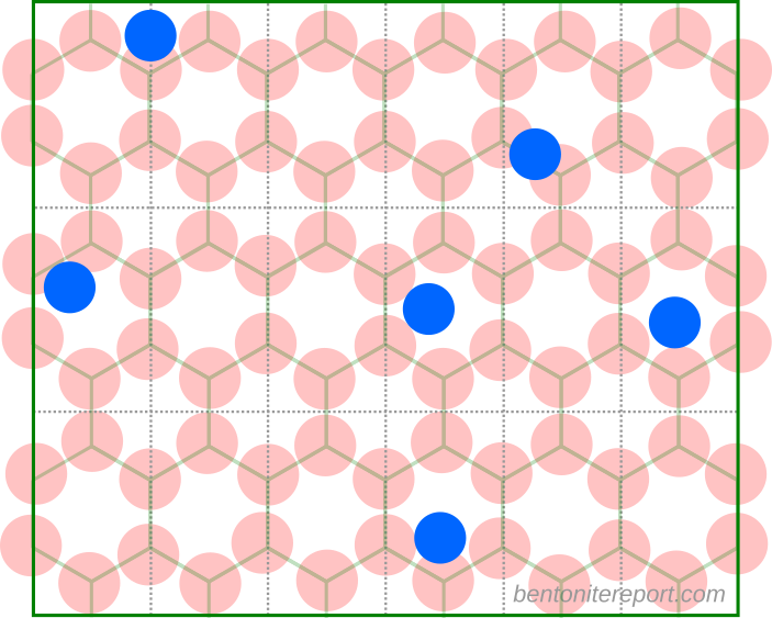
Clearly, there is room to accommodate all ions without running into the problems that was initially addressed by Stern’s model. Of course, solely accounting for the finite size of the ions — as is done in the simplest version of Stern’s model — is always well justified and will in principle improve the description. In particular, a pure diffuse layer model overestimates the capacitance of the surface. As shown in the table below, the introduction of an empty Stern layer “fixes” this problem.

\(c^\mathrm{ext}\) (M)	\(\psi^1\) (V)	\(c^1\) (M)	\(\psi^0\) (V)	\(K_\mathrm{Stern}\) (\(\mathrm{F}/\mathrm{m ^2}\))	\(K_\mathrm{DL}\) (\(\mathrm{F}/\mathrm{m ^2}\))
0.001	0.206	3.57	0.590	0.188	0.538
0.01	0.148	3.59	0.532	0.209	0.748
0.1	0.092	3.77	0.475	0.234	1.212
1	0.042	5.39	0.426	0.260	2.612

Here \(c^\mathrm{ext}\) is the concentration of the 1:1 salt far away from the surface, \(\psi^1\) and \(c^1\) denote the electrostatic potential and the counter-ion concentration, respectively, at the point where the diffuse layer begins (i.e. at the interface to the compact layer), and \(\psi^0\) is the electrostatic potential at the surface. \(K_\mathrm{Stern}\) denotes the corresponding capacitance as calculated from the Stern model, with the choice \(K_0 = 0.29 \;\mathrm{F/m^2}\). \(K_\mathrm{DL}\) is instead the capacitance as calculated from a pure diffuse layer model (in which case the surface potential has the value of \(\psi^1\)). In the calculations are assumed a montmorillonite surface charge of 0.111 \(\mathrm{C}/\mathrm{m ^2}\).

But to simply account for the finite size of the ions by means of an empty compact layer is not how the term Stern layer is used in the bentonite scientific literature. As mentioned, most bentonite researchers mean that parts of the rather sparse collection of ions on the surface interacts chemically (“specific sorption”, “chemisorption”). The question of whether Stern layers on montmorillonite basal surfaces are well motivated thus reduces to what arguments there are for more elaborate chemical mechanisms being active on these surfaces. And descriptions of specific sorption on basal surfaces are really all over the place.

Deshpande and Marshall (1959, 1961) claim that counter-ions are partitioned between (i) chemisorbed ions, which do not contribute to conductivity or activity, (ii) physisorbed ions in a Stern layer, which do not contribute to activity or D.C. conductivity, and (iii) diffuse layer ions, which contribute fully to activity and conductivity. If I interpret their numbers correctly, they state that about 75% — 80% of the counter-ions in pure K-montmorillonite are immobilized. Note that these authors mean that ions in the Stern layer are “physically” adsorbed, while the surface also has “chemically” adsorbed species. Thus, they use the term Stern layer for certain types of physisorption, while stating that ions also bond covalently to the surface.

Shainberg and Kemper (1966, 1967), on the other hand, model ions as either mobile in a diffuse layer or immobile in a Stern layer. They argue that covalently bound ions are “extremely unlikely”, and mean that ions in the Stern layer form “ion pairs” with the surface, as suggested earlier by Heald et al. (1964). They use this idea as a starting point for analyzing differences in exchange selectivity for different monovalent cations in montmorillonite. They claim that “about 20 to 50% of sodium are specifically adsorbed”.

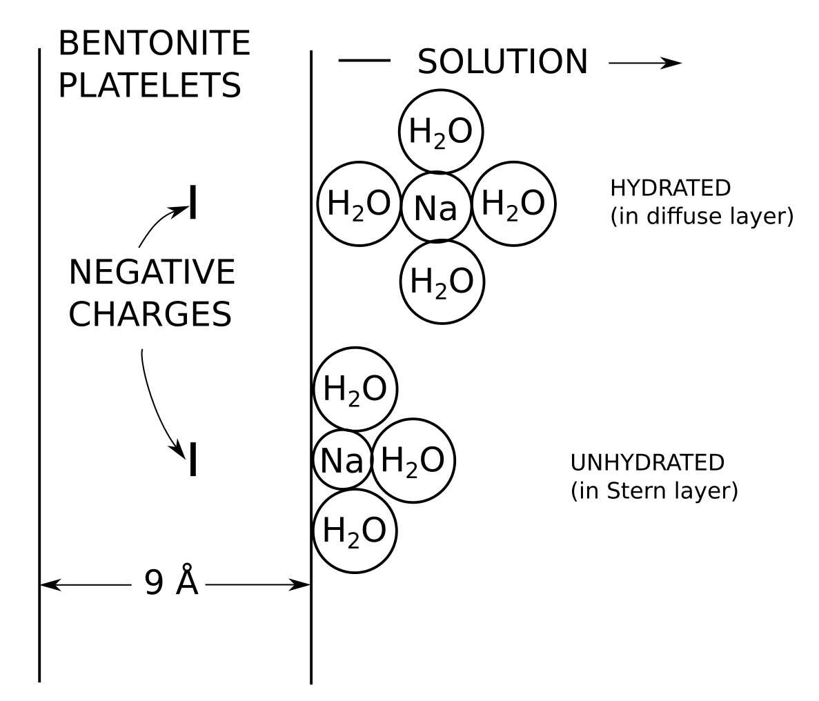
Note that Shainberg and Kemper, just like Deshpande and Marshall, assume Stern layer ions to be “physically” bonded to the surface (i.e. non-covalently), while having a completely different opinion on the presence of chemisorbed ions. Shainberg and Kemper (1966) provide a picture showing the conceptual difference between an ion in the Stern layer (“unhydrated”) and ions in the diffuse layer (“hydrated”) that looks very similar to this

In this context it may be worth to also mention the work of Low and co-workers. Low argued consistently that swelling pressure is not primarily related to the exchangeable ions — something that I strongly disagree with and that I commented briefly on in a previous blog post.⁴ Directly related to this view, these authors claim that the exchangeable ions for the most part do not dissociate from the surfaces, and in later papers they refer to such ions as being part of a Stern layer.

To me, all the above descriptions seem like little more than speculation. None of these authors discuss how or why e.g. sodium ions (!) are supposed to from ion pairs with a charge center buried far inside the montmorillonite layer, nor how or why they bond covalently with the basal surface. Nevertheless, both Low as well as Shainberg and Kemper seem to have influenced the writings of Sposito, who, in turn, has had quite a huge impact on contemporary descriptions of bentonite. In e.g. Sposito (1992), which specifically discusses montmorillonite (“smectite”), he writes

Despite the long history of continual investigation of the surface and colloid chemistry of smectites (van Olphen, 1977; Sposito, 1984), the structure of the electrical double layer at smectite surfaces and its influence on the rheological properties of smectite suspensions remain topics of lively controversy. One of the most contentious issues is the partitioning of adsorbed monovalent cations among the three possible surface species on the basal planes of smectite particles, such as montmorillonite (see, e.g., Low, 1981, 1987). […] [A] monovalent cation can be adsorbed on the basal planes by three different mechanisms: inner-sphere surface complexes, in which the cation desolvates and is captured by a ditrigonal cavity; outer-sphere surface complexes, in which the cation remains solvated but still is captured by a ditrigonal cavity and immobilized; and the diffuse-ion swarm, in which the cation is attracted to the basal plane, but remains fully dissociated from the smectite surface (Sposito, 1989a, Chap. 7).

The view conveyed here is that exchangeable ions do not interact with montmorillonite basal surfaces as if these, to a first approximation, are planes of uniform charge. Such interaction is only supposed to govern an outer diffuse layer (called a “diffuse-ion swarm” for unclear reasons), and ions are also supposed to interact with the surface by no less than two other “mechanisms”, related to the “ditrigonal cavities”.

Note that while Sposito acknowledges an ongoing “lively controversy” regarding how to describe montmorillonite basal surfaces, he specifies that this debate is limited to how to distribute the exchangeable ions among “three possible surface species.” But, as we will explore below, there is certainly no consensus within colloid chemistry that exchangeable ions are involved in complexation chemistry on the basal surfaces! (I therefore find this way of formulating the “controversy” quite dishonest, to be honest.) For reasons I can’t get my head around, descriptions of “inner-” and “outer-sphere complexes” on montmorillonite basal surfaces are anyway ubiquitous in modern bentonite literature. Let’s therefore take a closer look at how these are introduced.

“Inner-” and “outer-sphere” surface complexes

A description that hardly enlightens me is given in Sposito (1989)⁵

[The inner- and outer-sphere complexes] constitute the Stern layer on an adsorbent. […] The diffuse-ion swarm and the outer-sphere surface complex mechanisms of adsorption involve almost exclusively electrostatic bonding, whereas inner-sphere complex mechanisms are likely to involve ionic as well as covalent bonding. Because covalent bonding depends significantly on the particular electron configurations of both the surface group and the complexed ion, it is appropriate to consider inner-sphere surface complexation as the molecular basis of the term specific adsorption. Correspondingly, diffuse-ion screening and outer-sphere surface complexation are the molecular basis for the term nonspecific adsorption. Nonspecific refers to the weak dependence on the detailed electron configurations of the surface functional group and adsorbed ion that is to be expected for the interactions of solvated species.

Here, Sposito means that exchangeable ions bond covalently with the montmorillonite basal surface,⁶ in agreement with Deshpende and Marschall, and in disagreement with Shainberg and Kemper (we have one “extremely unlikely” and one “likely” for covalent bonding…). In contrast to Deshpende and Marschall, however, Sposito means that these “inner-sphere” complexes are part of the Stern layer. To confuse matters even more, Shainberg and Kemper assume their “unhydrated” construct (which corresponds structurally to an “inner-sphere” complex, see above figure) as being part of the Stern layer, but not part of any covalent bonding. Moreover, Shainberg and Kemper assume their “hydrated” construct (corresponding structurally to an “outer-sphere” complex, see above figure) to be part of the diffuse layer, while Sposito wants his “outer-sphere” complexes to be immobile and part of the Stern layer…

Given the above description (and others) it is hard to understand what the difference is supposed to be between an “outer-sphere” complex and an ion in the “diffuse-ion swarm”, other than that the former is simply claimed to be immobilized; both ions are said to interact with “exclusively electrostatic bonding”,⁷ both are classified as “nonspecific adsorption”, and both are fully hydrated. In my head, this is simply a recipe for achieving an overparameterized model description.

Sposito’s description also makes implicit statements about the montmorillonite basal surface: it contains “surface functional groups” whose specific electron configuration significantly influence covalent bonding, while being insensitive for the formation of “outer-sphere” complexes and the “diffuse ion-swarm”. In Sposito (1984) he suggests that the “functional groups” are groups of oxygen atoms on the surface of the montmorillonite particle (“ditrigonal cavities”) that qualifies as Lewis bases. The presence of atomic substitutions in the octahedral layer is supposed to enhance this Lewis base character

If isomorphic substitution of \(\mathrm{Al}^{3+}\) by \(\mathrm{Fe}^{2+}\) or \(\mathrm{Mg}^{2+}\) occurs in the octahedral sheet, the resulting excess negative charge can distribute itself principally over the 10 surface oxygen atoms of the four silica tetrahedra that are associated through their apexes with a single octahedron in the layer. This distribution of negative charge enhances the Lewis base character of the ditrigonal cavity and makes it possible to form complexes with cations as well as with dipolar molecules.

Note how completely different this whole description is compared to the original Gouy-Chapman conceptual view. Here is implied that montmorillonite basal planes⁸ cannot be described as a passive layer of charge, but that it is a fully reactive system, including covalent bonding mechanisms.

Frankly, I dismiss the above description of the montmorillonite surface as a Lewis base as pure speculation. I will gladly admit that I am a physicist rather than a chemist, and perhaps I am missing something obvious, but I really don’t see any argumentation behind this description. I am also under the impression that montmorillonite basal planes are relatively chemically stable — that is why they form in the first place, and that is also one reason for why we are interested in using bentonite for e.g. long-term geological waste storage. Furthermore, a meta-argument for dismissing this description is that in later publications we find statements like this, in Sposito (2004):

The \(\mathrm{Na}^+\) that are counterions for the negative structural charge developed as a result of isomorphic substitutions within the clay mineral layer tend to adsorb as solvated species on the basal plane (a plane of hexagonal rings of oxygen ions known as a siloxane surface) near deficits of negative charge originating in the octahedral sheet from substitution of a bivalent cation for \(\mathrm{Al}^{3+}\). This mode of adsorption occurs as a result of the strong solvating characteristics of Na and the physical impediment to direct contact between Na and the site of negative charge posed by the layer structure itself. The way in which this negative charge is distributed on the siloxane surface is not well known, but if the charge tends to be delocalized there, that would also lend itself to outer-sphere surface complexation.

So, 20 years after the surface chemistry of montmorillonite was described as if it was completely understood (Sposito, 1984), the way the negative charge distributes is now described instead as “not well known”… Furthermore, in contrast to earlier statements, the formation of an “outer-sphere complex” is here associated mainly with the hydration properties of sodium. But if the idea of a “surface functional group” is discarded — or at least downplayed — why should a hydrated ion near the surface be described as a surface complex at all?

We note that Sposito (2004) still seem to imply that the “outer-sphere surface complex” is localized and immobile (“adsorbed near deficits of negative charge”) But the evidence is vast that sodium, and several other ions, are quite mobile even in monohydrates (see below).

Deviations from the Gouy-Chapman model do not imply surface complexation

Authors that promote Stern layers on montmorillonite basal surfaces usually rely on the Gouy-Chapman model for describing the diffuse layer part. Lyklema, writing generally on colloid science, explicitly “defends” such an approach

In the following our discussion will be based on the rather pragmatic, though somewhat artificial, subdivision of the solution side of the double layer into two parts: an inner part, or Stern layer where all complications regarding finite ion size, specific adsorption, discrete charges, surface heterogeneity, etc., reside and an outer, Gouy or diffuse layer, that is by definition ideal, i.e. it obeys Poisson-Boltzmann statistics. This model is due to Stern following older ideas of Helmholtz and has over the decades since its inception rendered excellent services, especially in dealing with experimental systems.

Dzombak and Hudson (1995) express a similar attitude

Bolt and co-workers […] investigated in detail the application of the Gouy–Chapman diffuse-layer theory to ion-exchange processes. Their work demonstrated that consideration of electrostatic sorption alone is not sufficient to explain ion-exchange data and that chemisorption (or “specific” sorption) needs to be included in ion-exchange models.

It is not logically consistent to conclude that deviations from the Gouy-Chapman model implies that specific sorption “needs to be included”.⁹ On the contrary, introducing specific sorption to compensate for a certain model rather than for surface chemical reasons may, in my mind, be a recipe for an overparameterized disaster. I don’t get reassured by statements like this, also from Dzombak and Hudson (1995)

Surface complexation models can be extended to include diffuse-layer sorption. This approach permits their application in modeling the sorption of ions (such as monovalent electrolyte ions) that exhibit weak specific sorption. The generality of such an extended surface complexation approach together with the mathematical power of modern chemical speciation models offers the potential for accurate physicochemical modeling of ion exchange

Reasonably, a complex system may require complex models, but it is certainly dangerous in a modeling context to rely too heavily on “mathematical power” (I guess “numerical power” is the preferred phrase).¹⁰

Note that very different attitudes towards the Stern layer concept is found in the colloid science literature, where e.g. Evans and Wennerström (1999) describe it as an “intellectual cul de sac”.¹¹

One way of dealing with these difficulties is to say that the solution layer closest to a charged surface has properties so different from the bulk that it should be treated as a separate entity. This device was introduced in the 1930s by the German electrochemist Stern and the surface layer is commonly referred to as the Stern layer, whose properties are specified by a number of empirical parameters. It is the opinion of the authors of this book that the Stern layer concept is an intellectual cul de sac for the description of electrostatics in colloidal systems. One reason for this point of view is that from modern spectroscopic measurements we know molecular properties are not dramatically changed for a liquid close to a charged surface.

I find it quite perplexing that so many authors in the bentonite scientific community attribute any deviation from the Gouy-Chapman model solely to surface-related mechanisms. The Gouy-Chapman model treats both ions (point particles) and water (a dielectric continuum) in a very simplified manner, and it is clear that “specific ion” effects are ubiquitous, also in systems that lack surfaces. Addressing differences in e.g. selectivity coefficients without considering ion polarizability and hydration, while postulating the existence of localized sorption “sites”, can, to my mind, only lead to incorrect descriptions.

The Poisson-Boltzmann equation is a mean field approximation

Note also that the Poisson-Boltzmann equation — which underlies the Gouy-Chapman model — is only approximate. It is derived by assuming that the electrostatic potential experienced by any ion is the average potential from all other ions (and surfaces). More accurately, the ion distribution around a given ion deviates from the average, as a direct consequence of the presence of the central ion.

Including these ion-ion correlation effects makes the mathematical description considerably more complex. But with the advent of sufficiently powerful computers and algorithms, the electric double layer has been solved basically “exactly”. The “exact” solution may differ strongly from the Poisson-Boltzmann solution, with increasing concentrations towards the surfaces (and consequently a lowering of interlayer midpoint concentrations), and an explicit attractive electrostatic force between the two halves of an interlayer. Using Monte Carlo simulations, Guldbrand et al. (1984) demonstrated that with divalent counter-ions these effects are so large that the system becomes net attractive at a certain interlayer distance, in qualitative disagreement with the Poisson-Boltzmann solution. This effect, which has been thoroughly studied since the 80s, and which we have discussed in several posts on this blog, is the prevailing explanation e.g. for the limited swelling of Ca-montmorillonite.

The lesson here is that observed deviations from predictions of the Poisson-Boltzmann equation not automatically can be taken as evidence for additional active system components, and certainly not as evidence for specific sorption. Note that limited swelling in divalent montmorillonite is explained by the ions being diffusive, not that they are sorbed and immobilized. I cannot overstate the importance of this insight.

It boggles my mind that the entire research area on ion-ion correlations in colloidal systems seems to have made no significant impact on parts of the bentonite scientific community; I seldom find references to works on ion-ion correlation, and when I do it’s quite confused. E.g. Sposito (1992) means that the formation of “quasicrystals”¹² is due to “outer-sphere” complexes

The best known example of a montmorillonite quasicrystal is that comprising stacks of four to seven layers. \(\mathrm{Ca}^{2+}\) ions, solvated by six water molecules (outer-sphere surface complex), serve as molecular “cross-links” to help bind the clay layers together through electrostatic forces.

Sure, the ion-ion correlation effect that prevents Ca-montmorillonite from exfoliating is of electrostatic origin, but it is not related to “cross-links” or surface complexes. Sposito furthermore continues by claiming that “even […] Na-montmorillonite” forms “quasicrystals”. Such claim cannot be supported by ion-ion correlation — on the contrary, ion-ion correlation explains why Ca-montmorillonite forms “quasicrystals”, while Na-montmorillonite does not. It is thus relatively clear that Sposito do not refer to ion-ion correlation in the above statement. At the same time, later in the same publication he cites Kjellander et al. (1988) on going beyond the mean-field treatment of the Poisson-Boltzmann equation, and even claims that the Gouy-Chapman model is “completely inaccurate” for systems containing divalent ions. I can only conclude that this is a quite confused description.

Finite-size effects of water molecules

With focus on the first molecular layers at a solid interface, it is clear that finite-size effects of water molecules — which are not treated in the Gouy-Chapman model — reasonably influences the resulting ion distribution. This influence is manifested both as a steric effect — there can only be a discrete number of water molecules between the ion and the surface — and as an effect of how strongly a certain ion is hydrated.

Water molecules are treated explicitly e.g. in molecular dynamics (MD) simulations of montmorillonite/water interfaces, and here are results from simulating a three water-layer interlayer of Na-montmorillonite, from Hedström and Karnland (2012)¹³

Sodium is seen to accumulate “between” the water layers; in the above illustration we have also included schematic illustrations of the molecular configurations, as conceived by Shainberg and Kemper (1966) (shown earlier). As stated earlier, Shainberg and Kemper (1966) refer to these as “hydrated” and “unhydrated”, but they are clearly the same type of configurations that e.g. Sposito (1992) and Dzombak and Hudson (1995) call “outer-” and “inner-sphere” complexes.

While the above mentioned authors mean that these “complexes” involve specific interactions between ions and surface, the MD simulation suggests that such structures are mainly a consequence of the finite-size of the molecules and ions. In particular, the MD results do not support the idea that these structures depend critically on a specific, non-electrostatic, ion–surface interaction. Indeed, the simulations explicitly treat also the atoms of the montmorillonite layer, which could make it difficult to judge whether the appearance of “complexes” mainly is related to water–ion or ion–surface interactions. But note that Hedström and Karnland (2012) simulate two different systems: one where the montmorillonite charge is put on specific atoms in the octahedral sheet (Mg for Al substitutions), and one where it is distributed on all Al atoms (as a fraction of the elementary charge). Both systems have essentially an identical atomic configuration in the interlayer, which strongly suggest that no critical ion–surface interaction is involved in forming “outer-” and “inner-sphere complexes” (i.e. they really are not surface complexes). I am not aware of any published simulation where the basal surface is represented as a uniform sheet of charge while water molecules are treated explicitly, but I am convinced that “outer-” and “inner-sphere complexes” would appear also in such a simulation.

Regarding MD simulations of montmorillonite interlayers, you can also simply observe them to convince yourself that the counter-ions are not in any reasonable sense immobilized. These types of simulations are routinely used to calculate (quite significant) interlayer diffusion coefficients, for crying out loud!

Experimental evidence of counter-ion mobility

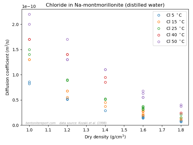
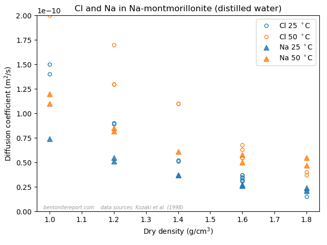
A final argument for why Stern layers on montmorillonite basal surfaces are unjustified is the vast amount of empirical evidence of counter-ion mobility. We have discussed several diffusion studies in earlier blog posts that show that many ions (Na, Cl, K, Sr, I, Cs, Ca,…) have a significant mobility even in very dense systems, dominated by bi- or monohydrated interlayers. In the previous post, we brought up the following result

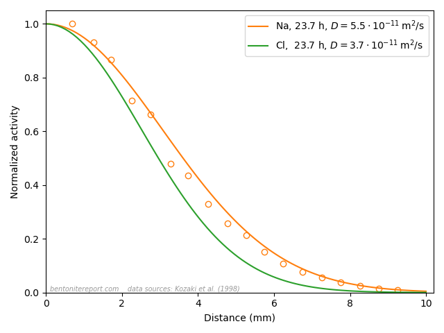
This figure shows the resulting concentration profiles in two diffusion experiments where sodium and chloride tracers, respectively, have diffused from an initial planar source for the same amount of time (23.7 h), in samples of pure Na-montmorillonite of dry density 1.8 \(\mathrm{g/cm^3}\), equilibrated with deionized water. This result was used previously to dismiss the ludicrous idea that these two ions are supposed to migrate in separate parts of the pore volume, exposed to completely different mechanisms. In the same vein, this result can be used to dismiss the idea of a Stern layer on basal surfaces.

Sodium, which is universally acknowledged to reside in the interlayers, is here demonstrated to diffuse just fine in bi- and monohydrated interlayers. As chloride, which also resides in the interlayers (despite all talk of “anion-accessible porosity”), behave essentially identical, it is quite far-fetched to assume any significant surface complexation mechanism. And anyone who argues for that these tracers actually do not diffuse in the interlayers should be reminded of the seeming “uphill” diffusion experiment,¹⁴ which is performed at even higher density, and where the “uphill” diffusion direction once and for all proves that the transport occurs in interlayers.

Strangely, many authors nowadays seem to promote both Stern layers and interlayer mobility in bentonite. Various simulation codes has been modified for this possibility, and there are several examples of researchers pointing out a possibility of “Stern layer diffusion”. I think these authors should carefully examine their chain of assumptions: Surface complexation in a Stern layer (i.e. sorption) is initially suggested to explain e.g. why breakthrough times in cation through-diffusion tests are relatively long as compared with the steady-state flux (i.e. why “\(D_e\)” can be considerably larger than”\(D_a\)”). With evidence for that the “sorbed” ions actually dominate the mass transfer, the sorption mechanism is not reconsidered, but yet another mechanism is suggested: Stern layer mobility… Reasonably, such an approach is not adequate for developing models; researchers employing it should critically consider the intended purpose of a Stern layer component.

Counter-ion mobility is also related to swelling pressure. Bentonite swelling pressure is difficult to describe generally, and I have written a whole series of blog posts on the subject, but it is clear that measured swelling pressures in e.g. moderately dense Na- and Li-montmorillonites is quite well described by the Poisson-Boltzmann equation. As this set of conditions (not too dense clay, simple monovalent ions) are exactly those for which we expect the Poisson-Boltzmann equation to be adequate, this is a strong indication that all counter-ions contribute to the pressure.¹⁵ Also, the limited swelling in e.g. Ca-montmorillonite, as previously discussed, is explained by ion-ion correlation effects where all ions are included in the diffuse layer.

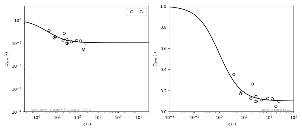
Finally, we can take a look at salt exclusion from compacted bentonite. The magnitude of salt exclusion is directly related to the amount of mobile counter-ions. Thus, if most of the counter-ions were immobilized in a Stern layer, bentonite should show small exclusion effects. In contrast, the empirical results for e.g. chloride exclusion in sodium dominated bentonite indicate, again, that all counter-ions are part of a diffuse layer.

This diagram shows the relative amount of chloride in the bentonite as a function of \(c^\mathrm{ext}/c_\mathrm{IL}\), where \(c^\mathrm{ext}\) is the external salt concentration and \(c_\mathrm{IL}\) is the amount exchangeable cations, expressed as a monovalent interlayer concentration. The experimental data is from Van Loon et al. (2007), which we reevaluated and examined in detail in a previous blog post. The lines are the result from applying the “ideal” Donnan formula with various amounts of the counter-ions assumed diffusive. For details on Donnan theory, see this blog post.

Although the experimental data show considerable scatter, there is nothing in this plot that suggests that a fraction of the counter-ions are immobilized. And the quality of this data is certainly good enough to directly dismiss models that assume that the major part of ions are immobilized in a Stern layer.

Footnotes

[1] I find it quite frustrating that many descriptions in the literature only refer abstractly to “mineral surfaces” rather than specifically addressing montmorillonite. At the same time it is often clear from the context that statements regarding “mineral surfaces” should be understood as applicable to montmorillonite basal surfaces. I would much appreciate if researchers promoting Stern layers on basal surfaces would provide descriptions for specific systems, e.g. pure Na-Ca-montmorillonite.

[2] Otto Stern is a fascinating character in the history of science, most famous for the Stern-Gerlasch experiment, that helped pave the way for quantum mechanics. I highly recommend this lecture by the late Sandip Pakvasa. An example of its contents:

A note on Stern’s style of working: He always had a cigar in one hand, and he left actual work with hands to others, as he did not trust his own manual dexterity! […] He described the beneficial effects of a large wooden hammer that he kept in his lab and used it to threaten the apparatus if it did not behave! (apparently it worked!)

[3] Note that di-valent counter-ions would be even more sparsely distributed than this.

[4] It may be worth discussing my objections against the work of Low and co-workers in more detail in a future blog post.

[5] This is a general discussion on sorption on mineral surfaces, and is cited from the second edition of the book (2008). There is also a “Thired” edition.

[6] This particular description is general (for “adsorbents”), but since Sposito, as well as a large part of the contemporary bentonite scientific community, claim that “inner-sphere” complexes are present on montmorillonite basal surfaces, we can conclude that they mean that covalent bonding occur on such surfaces.

[7] Sure, the full quotation is “almost exclusively electrostatic bonding”, but what is a reader supposed to do with that? Such vague and sloppy scientific writing annoys me.

[8] Again, the discussion is on general “mineral surfaces”, but from other writings it is clear that this is supposed to apply to the montmorillonite basal surface.

[9] I furthermore don’t believe that “Bolt and co-workers” concluded that specific sorption “needs” to be included, but that this rather is an interpretation made by Dzombak and Hudson themselves. Bolt considered and downplayed the Stern Layer already in the mid 50s, and although he indeed has expressed positive attitudes (seriously, these guys just write too much!), he continued to downplay its significance in e.g. Bolt (1979), writing “In conclusion it appears justified to assume that for homoionic clays saturated with common ions, if hydrated, the Stern layer will be an “empty” Stern layer according to the terminology of Grahame (1947).”

[10] Note also that the perspective in this quotation is that specific sorption models can be complemented with diffuse layer features — i.e. the existence of sorption “sites” is assumed a priori. But Dzombak and Hudson (1995) never really discuss the nature of such “sites” on montmorillonite basal surfaces, but rely on Sposito’s speculations about “inner-” and “outer-surface” complexes.

[11] Note that Stern’s original paper actually is from 1924. I also suspect that Stern would object to being labeled an “electrochemist”.

[12] The terminology here is quite messy, and other authors may use other terms such as “tactoids”, see this post for a further discussion.

[13] This study was thoroughly discussed in a blog post on MD simulations and anion exclusion.

[14] Anyone making this argument should also provide a plausible suggestion for where a significant non-interlayer pore structure is located at these extreme densities.

[15] The pressure in these types of calculations can be related to the interlayer midpoint concentration. But this does not mean that not all counter-ions are involved in the process.

Post-publication review: Tournassat and Steefel (2015), part I

Leave a reply

Here’s an opinion: The compacted bentonite research field is currently in a terrible state.

After a period away, I’ve recently begun catching up on newly published research in this field. With a fresh perspective, yet still influenced by writing over 30 long-reads over the past years, I can’t help but wonder: what is the problem? Why are a majority of researchers stuck with a view of bentonite¹ that essentially makes no sense? And why has this view been the mainstream for decades now?

I get how this might come across: a solitary man ranting on a blog, criticizing an entire research field in less-than-perfect English. I probably smell bad and have some wild ideas about why General Relativity is wrong as well. But what I’m aiming for with this blog is simply a platform to present an alternative to the mainstream, primarily because it annoys me as a science-minded person how absurd this view is.² I understand that I will likely struggle to convince anyone who is already invested in this view, but I’m trying to put myself in the shoes of e.g. someone entering this field for the first time.

For these reasons, I will try something a little new here: reviewing already published papers. I have touched on this in various forms before, but then usually with a broader topic in mind. Now I intend to critically assess specific publications from the outset. As a first publication to review in this way, I have chosen “Ionic Transport in Nano-Porous Clays with Consideration of Electrostatic Effects” (Tournassat and Steefel, 2015), for the following reasons

It is published in “Reviews in Mineralogy & Geochemistry”, which claims that “The content of each volume consists of fully developed text which can be used for self-study, research, or as a text-book for graduate-level courses.” If anyone aims to learn about ion transport in bentonite from this publication, I would certainly recommend to also consider this review.
It is a quite comprehensive source for many of the claims of the contemporary mainstream view that I have described in earlier blog posts. I guess it makes sense for a publication in “Reviews in Mineralogy & Geochemistry” to reflect the typical view of a research field.
It considers the seeming uphill diffusion effect that I recently commented on. The effect is as misunderstood in this publication as it is in Tertre et al. (2024).
It is published as open access. The article is thus accessible to anyone who wants to check the details.

I will use the abbreviation TS15 in following to refer to this publication.

Overview

The article covers 38 journal pages (+ references) and includes quite a lot of topics. At the highest level of headings, the outline look like this

Introduction (p. 1 — 2)
Classical Fickian Diffusion Theory (p. 2 — 9)
Clay mineral surfaces and related properties (p. 9 — 17)
Constitutive equations for diffusion in bulk, diffuse layer, and interlayer water (p. 17 — 23)
Relative contributions of concentration, activity coefficient and diffusion potential gradients to total flux (p. 24 — 28)
From diffusive flux to diffusive transport equations (p. 28 — 33)
Applications (p. 33 — 37)
Summary and Perspectives (p. 37 — 38)

Given the quite large scope of TS15, I will present this review in parts, with this first part focusing on the introduction and the section titled “Classical Fickian Diffusion Theory”.

“Introduction”

I find it remarkable that the authors use terms like “clays” and “clay minerals” when speaking of properties such as “low permeability”, “high adsorption capacity” and “swelling behavior”, and of applications such as nuclear waste storage. I mean that using such general terms here is too broad, as the article focuses solely on systems with swelling/sealing ability. Such an ability is generally connected with a significant cation exchange capacity. Here, I will refer to such systems as “bentonite”, although I am aware that I use the term quite sloppily. But I think this is better than to refer to the components as general “clay minerals” — I don’t think anyone consider it a good idea to e.g. use talc or kaolinite as buffer materials in nuclear waste repositories. Moreover, most of the examples considered in the article are systems that can be described as bentonite. Given the title of the article I also expect a definition of “nano-porous clays”. It is not given here, and the term is actually not used at all in the entire text! (Except one time at the very end.)

After providing a brief overview of the application of (sealing) clay materials, the introduction takes, in my opinion, a rather drastic turn (it happens without even changing paragraphs!).

Clay transport properties are however not simple to model, as they deviate in many cases from predictions made with models developed previously for “conventional” porous media such as permeable aquifers (e.g., sandstone). […] In this respect, a significant advantage of modern reactive transport models is their ability to handle complex geometries and chemistry, heterogeneities and transient conditions (Steefel et al. 2014). Indeed, numerical calculations have become one of the principal means by which the gaps between current process knowledge and defensible predictions in the environmental sciences can be bridged (Miller et al. 2010).

I think the first sentence is too subjective and general. Given the above discussion, here the term “clay transport properties” can cover a million things, if read at face value. Are all of them difficult to model? Also, something does not have to be more difficult just because it deviates from the “convention”. I would argue that several aspects of bentonite actually make it easier to model than, say, sandstone. Advective processes, for example, can often be neglected in compacted bentonite.

I find the statement regarding the advantage of reactive transport models highly problematic. Not only does it read more like an advertisement for the authors’ own tools than “fully developed text for self-study”, but the authors also seem ignorant of issues like the dangers of overparameterization (a theme that will recur).

“Classical Fickian Diffusion Theory”

As the title of the next section is “Classical Fickian Diffusion Theory,” a reader expects a discussion focused solely on diffusive process, especially when the immediate subtitle reads “Diffusion Basics.” I therefore find it peculiar that this section actually presents the traditional diffusion-sorption model, which describes a combination of diffusion and sorption processes. The model is summarized in eq. 10 in TS15

\begin{equation} \frac{\partial c}{\partial t} = \frac{D_e} {\phi + \rho_dK_D} \nabla ^ 2 c \end{equation}

where \(c\) is the “pore water” concentration of the considered species, \(D_e\) its “effective diffusivity”, \(K_D\) the sorption partition coefficient, \(\rho_d\) dry density, and \(\phi\) porosity.³ For later considerations we also note that TS15 define the denominator on the right hand side as the “rock capacity factor”, \(\alpha = \phi + \rho_dK_D\).

I find it particularly odd that two of the fundamental assumptions of this specific model are essentially left uncommented, namely that sorbed ions are immobilized and that the pores contain bulk water. Instead, the authors appear to question the assumption of Fickian diffusion in the context of clay systems, i.e. that diffusive fluxes are assumed proportional to corresponding aqueous concentration gradients.

This section aims, as far as I can see, to point out shortcomings in the description of diffusion in bentonite, and to motivate further model development. But it should be clear from the outset that using the traditional diffusion-sorption model as the basis for such an endeavor is doomed to fail. The reason for this failure is not due to assuming Fickian diffusion, but due to the other two model assumptions; it has long been demonstrated that exchangeable ions are mobile, and the notion that compacted bentonite contains mainly bulk water is absurd.

After the traditional diffusion-sorption model has been presented, it is evaluated by investigating how it can be fitted to tracer through-diffusion data (this is restatement of original work of Tachi and Yotsjui (2014)). Not surprisingly, it turns out that fitted diffusion coefficients may be unrealistically large. This is of course a direct consequence of the incorrect assumption of immobility in the traditional diffusion-sorption model. TS15 also appear to dismiss the model, saying

This result […] is not physically correct and points out the inconsistency of the classic Fickian diffusion theory for modeling diffusion processes in clay media.

I am bothered, though, that they keep using the phrase “classic Fickian diffusion theory”, which inevitably focuses on the Fickian aspect rather than on the obviously incorrect assumptions of the chosen model. Also, rather than simply concluding that the model is incorrect, TS15 continues⁴

[T]he large changes of \(\mathrm{Cs}^+\) diffusion parameters as a function of chemical conditions (\(D_{e,\mathrm{Cs}^+}\) decreases when the ionic strength increases […]) highlight the need to couple the chemical reactivity of clay materials to their transport properties in order to build reliable and predictive diffusion models.

There is no rationale for such a conclusion. I don’t even completely understand what “couple the chemical reactivity of clay materials to their transport properties” mean. Isn’t that what the traditional diffusion-sorption model attempts? What unrealistic \(D_e\) values actually highlights is simply that one should not use a model that assumes immobilization of “sorbed” ions.

To make things worse, TS15 describe the seeming uphill diffusion test and comment

However, the experimental observations were completely different: \(^{22}\mathrm{Na}^+\) accumulated in the high NaCl concentration reservoir as it was depleted in the low NaCl concentration reservoir, evidencing non-Fickian diffusion processes.

This is plain wrong. As explained in detail in an earlier post, the diffusion process in the “uphill” test is certainly Fickian. What the test demonstrates is, again, that “sorbed” ions are not immobile.

TS15 also comment on the results of fitting the model to anion tracer through-diffusion data. Here, as is well known, the fitted “rock capacity factor” \(\alpha = \phi + \rho_dK_D\) becomes significantly lower than the porosity \(\phi\). From the perspective of the traditional diffusion-sorption model, this is completely infeasible, as it implies a negative \(K_D\). But rather than simply dismissing the model, TS15 state

The lower \(\alpha\) values for anions than for water indicate that anions do not have access to all of the porosity.

Also this is incorrect. The porosity⁵ is an input parameter rather than a fitting parameter in the traditional diffusion-sorption model. When claiming that a small value of \(\alpha\) indicates a decreased porosity, TS15 reinterpret the parameter, on the fly, in terms of a completely different model: the effective porosity model. This model has not been mentioned at all earlier in the article.⁶

As has been discussed earlier on the blog, the effective porosity model can be fitted to anion tracer through-diffusion data, but now we need to keep track of two different models in the evaluation (something that TS15 do not). Moreover, these two models (the traditional diffusion-sorption and the effective porosity models) are incompatible. But TS15 continue by saying

This result is a first direct evidence of the limitation of the classic Fickian diffusion theory when applied to clay porous media: it is not possible to model the diffusion of water and anions with the same single porosity model. The observation of a lower \(\alpha\) value for anions than for water led to the development of the important concept of anion accessible porosity […]

This is a terrible passage. To begin with, the “Fickian” aspect is also here implied as the problem. But the reason for why the traditional diffusion-sorption model cannot be fitted to anion tracer through-diffusion data is of course because this model assumes the entire pore space to be filled with bulk water. Further, it’s hardly comprehensible what the authors mean by “it is not possible to model the diffusion of water and anions with the same single porosity model”. I think they simply mean that for water you must choose \(\alpha = \phi\), while for anion through-diffusion you instead must “choose” \(\alpha < \phi\). But the result \(\alpha < \phi\) should only lead to the conclusion that the traditional diffusion-sorption model cannot in any reasonable sense be fitted. A favorable reading of this passage is to assume that the authors actually mean that the effective porosity model can only be fitted to anion and water tracer through-diffusion data by using different values of the (effective) porosity, and that any “rock capacity factor” should not appear in this discussion.

Finally, the last sentence gives me headache. Rather than being an “important concept”, I mean that the idea of an “anion accessible porosity” has caused tremendous damage to the development of the bentonite research field for several decades now. We have earlier discussed on the blog that the whole idea of “anion accessible porosity” is based on misunderstandings. We have also demonstrated that the effective porosity model is not valid, even though it can be fitted to anion tracer through-diffusion data. A simple way to see this is to consider closed-cell diffusion data rather than through-diffusion data. Closed-cell tests are simpler than through-diffusion tests, as they don’t involve interfaces between clay and external solutions. We can e.g. take a look at the vast amount of diffusion coefficients for chloride in montmorillonite, presented in Kozaki et al. (1998).

There are in total 55(!) values, corresponding to 55(!) separate tests. These have been systematically varied with respect to density and temperature, but all of them were performed on montmorillonite equilibrated with distilled water. From the perspective of the effective porosity model, the effective porosity in such a system should be minute, perhaps even strictly zero; effective porosities evaluated from chloride through-diffusion tests are well below 1% even at a background concentration as large as 10 mM. Thus, if the idea of “anion accessible porosity” was reasonable, we’d expect extremely low values of the chloride diffusion coefficient in the above plot.⁷ We’d perhaps also expect a threshold behavior, where chloride diffusivity basically vanishes above a certain density. But this is not at all the behavior: chloride is seen to diffuse just fine in all 55(!) tests, with temperature- and density dependencies that seems reasonable for a homogeneous system. Moreover, chloride behaves very similarly to e.g. sodium, as seen here

Here the sodium data is from Kozaki et al. (1998),⁸ and it has also been measured in montmorillonite equilibrated with distilled water.

The effective porosity model and the notion of “anion accessible porosity” can consequently be dismissed directly, by comparing with simpler tests than what is done in TS15. The reason that the effective porosity model can be fitted to anion through-diffusion data must be attributed to a misinterpretation of such tests, as they involve also interfaces to external solutions. At least to me it is completely clear that what many researchers interpret as an effective porosity is actually effects of interface equilibrium.

If TS15 were serious about evaluating bentonite diffusion processes in this section I think they should have done the following:

Discuss the assumptions of ion immobility of sorbed ions and bulk pore water when presenting the traditional diffusion-sorption model. Moreover, they should not call this “Classical Fickian Diffusion Theory”.
Also present and discuss the effective porosity model, as they obviously use it in their evaluations. They actually even seem to promote it! And it is as “Fickian” as the traditional diffusion-sorption model.
Evaluate the models using closed-cell data to avoid misinterpretations arising from complications at bentonite/external solution interfaces.
Conclude that the traditional diffusion-sorption model is not valid for bentonite, and that this is because of the assumptions of immobility of sorbed ions and bulk pore water.
Conclude that the effective porosity model is not valid for bentonite, and that the notion of “anion accessible porosity” is flawed.

Instead, we get a quite confused and incomplete description, mixed with entirely inaccurate statements. In the end, it is difficult to understand what the takeaway message of this section really is. A reader is left with an impression that there is some problem with the “Fickian” aspect of diffusion, but nothing is spelled out. We have also been hinted that “anion accessible porosity” is important, without really having been introduced to the concept/model.

The section ends with the following passage

The limitations of the classic Fickian diffusion theory must find their origin in the fundamental properties of the clay minerals. In the next section, these fundamental properties are linked qualitatively to some of the observations described above.

If “classic Fickian diffusion theory” here is interpreted as “the traditional diffusion-sorption model” (which is literally what has been presented), the first sentence is both incorrect and trivial at the same time. The traditional diffusion-sorption model does not have “limitations” — it is fundamentally incorrect as a model for bentonite. The reason for this is that exchangeable ions are not immobile and that bentonite does not contain significant amounts of bulk water. Both of these reasons can be linked to “fundamental properties” of some specific clay minerals.

But it is clear that TS15 also have vaguely promoted the concept of “anion accessible porosity” and the effective porosity model. Are these not included in “the classic Fickian diffusion theory”? If not, why then is a model that assumes sorption and immobilization?

How can it not be immediately obvious to everyone that the diffusion process is much simpler than the contemporary descriptions?

As we have brought up the data from Kozaki et al. (1998), I would like to end this blog post by further considering actual profiles of chloride and sodium diffusing in montmorillonite.

This figure shows the corresponding normalized concentration profiles after 23.7 hours in closed-cell tests performed at \(50\;^\circ\mathrm{C}\) in Na-montmorillonite at dry density \(1.8 \;\mathrm{g/cm^3}\) that has been equilibrated with distilled water. In the case of sodium, both the profile evaluated from Fick’s second law (orange line) and measured values (circles) are plotted. In the case of chloride, no measured values are available, but the value of the diffusion coefficient is the result of fitting Fick’s second law (green line) to such data.

From the perspective of the traditional diffusion-sorption model, the sodium profile is supposed to represent the combined result of ions diffusing in bulk water, at a rate many orders of magnitude larger than in pure water, while being strongly retarded due to sorption onto “the solid” (where the ions are immobile). This is clearly nonsense, and something that I think TS15 actually tries to communicate.

From the perspective of the effective porosity model, on the other hand, the chloride profile is supposed to be the result of the ion diffusing in an essentially infinitesimal fraction of the pore volume, which magically is perfectly interconnected in all samples on which such tests are conducted. This is of course just as nonsensical as the above interpretation of the sodium profile, but in this case TS15 appear to promote the model (the “important concept of anion accessible porosity”).

Note that these two simple ions, at the end of the day, diffuse very similarly (please stop reading for a moment and contemplate the above plot). If sodium and chloride actually migrate in completely different domains and are subject to completely different physico-chemical processes, this “coincident” would be more than a little weird. Especially given that the two ions show similar diffusive behavior across a wide range of densities. To me, this simple observation makes it evident that ion diffusion in bentonite at the basic level is much simpler than what is suggested by the contemporary mainstream view. I mean that it is completely obvious that all ions in bentonite diffuse in the same type of quite homogeneous domain. And since it cannot be argued that the pore volume is dominated by anything other than interlayers at 1.8 g/cm³, this homogeneous domain is the interlayer domain at any relevant density. The evidence has been available for at least 25 years (in fact much longer than that). How can this be difficult to grasp?

Update (250213): Part II of this review is found here.

Footnotes

[1] By “bentonite” I here mean any type of smectite-rich system with a significant cation exchange capacity.

[2] The irony is that the “alternative” in a broader perspective is more mainstream than the “mainstream” view. I basically propose to obey the laws of thermodynamics.

[3] I have simplified the notation here somewhat compared with how it is written in TS15. As many others, TS15 call this equation “Fick’s second law” (via their eq. 4), which is not correct. Fick’s laws refer strictly to pure diffusion processes. However, the equation has the same form as Fick’s second law, if \(D_e/(\phi + \rho_d K_D)\) is treated as a single constant (often referred to as the apparent diffusivity).

[4] This behavior is of course not unique for cesium; I don’t know why TS15 focus so hard on that ion here.

[5] “Porosity” is a volume ratio. I’m not a fan of that the word has also begun to mean “pore space” in the bentonite scientific literature.

[6] In fact, \(\alpha\) has earlier in the article been unambiguously related to sorption:

If the species \(i\) is also adsorbed on or incorporated into the solid phase, then it is possible to define a rock capacity factor \(\alpha_i\) that relates the concentration in the porous media to the concentration in solution

[7] That the diffusivity is much too large for an effective porosity interpretation to make sense can also be seen from invoking Archie’s law, which is quite popular in bentonite scientific papers.

\begin{equation} D_e = \epsilon_\mathrm{eff}^n D_0\end{equation}

Here \(D_0\) is the diffusivity in pure bulk water, which is about \(2\cdot 10^{-9} \;\mathrm{m^2/s}\) for chloride. Using the popular choice \(n \approx 2\) and choosing e.g. \(\epsilon_\mathrm{eff} = 0.001\) (most probably an overestimation when using distilled water), we get

\begin{equation} D_0 = (5.1\cdot 10^{-11} \;\mathrm{m^2/s})/0.001 = 5.1\cdot 10^{-8} \;\mathrm{m^2/s}\end{equation}

This is more than twenty times the actual value for \(D_0\). (\(D_e = 5.1\cdot 10^{-14} \;\mathrm{m^2/s}\) is evaluated from Kozaki’s data at \(1.4 \;\mathrm{g/cm^3}\) and \(25\;^\circ\mathrm{C}\))

[8] Note! This publication is different from the chloride study.

Sorption part IV: What is K_d?

Leave a reply

Measuring K_d

Researchers traditionally measure sorption on montmorillonite in batch tests, where a small amount of solids is mixed with a tracer-spiked solution (typical solid-to-liquid ratios are \(\sim 1 – 10\) g/l). After equilibration, solids and solution are usually separated by centrifugation and the supernatant is analyzed.

This procedure evidently counts tracer cations that reside in diffuse layers as sorbed. But tracer ions may also sorb due to other mechanisms, in particular due to bonding on specific surface hydroxyl groups, on the edges of individual montmorillonite layers. These different types of “sorption” are in the clay literature usually referred to as “cation exchange” and “surface complexation”, respectively.

The amount of tracer “sorbed” in the ways just described is quantified by the distribution coefficient \(K_d\), defined as

\begin{equation} s = K_d\cdot c_\mathrm{eq} \end{equation}

where \(s\) denotes the amount of tracers “on the solids”, and \(c_\mathrm{eq}\) is the corresponding equilibrium concentration in the aqueous phase. As the amount “on the solids” can be inferred from the amount of tracers that has been removed from the initial solution, we can evaluate \(K_d\) from

\begin{equation} K_d = \frac{\left ( c_\mathrm{init} – c_\mathrm{final} \right ) \cdot V_\mathrm{sol}} {c_\mathrm{final}\cdot m_\mathrm{s}} \end{equation}

where \(c_\mathrm{init}\) is the initial tracer concentration (i.e. before adding the clay), \(c_\mathrm{final}\) is the tracer concentration in the supernatant, \(V_\mathrm{sol}\) is the solution volume, and \(m_s\) is the mass of the solids.

If the purpose of a study is solely to quantify the amount of tracer “on the solids”, it is adequate to define sorption as including both “cation exchange” and “surface complexation”, and to use \(K_d\) as the measure of this sorption. However, if our main concern is to describe transport in compacted bentonite, \(K_d\) is a rather blunt tool, since it quantifies both ions that dominate the transport capacity (“cation exchange”), and ions that are immobile, or at least contribute to an actual delay of diffusive fluxes (“surface complexation”).

A good illustration of this problem is the traditional diffusion-sorption model, which incorrectly assumes that all ions quantified by \(K_d\) are immobilized. In earlier blog posts, we have discussed the consequences of this model assumption, and the empirical evidence against it. A complication when discussing sorption is that researchers often “measure” \(K_d\) by fitting the traditional diffusion-sorption model to data — although the model is not valid for compacted bentonite.

Moreover, when evaluating \(K_d\) in batch tests, or when using this parameter in models, authors assume that the solids are in equilibrium locally with a bulk water phase. But there is no compelling evidence that such a phase exists in compacted water saturated bentonite. On the contrary, several observations strongly suggest that compacted bentonite lacks significant amounts of bulk water. This, in turn, suggests that \(K_d\) actually quantifies the equilibrium between a bentonite sample and an external solution.

Indeed, even in batch tests is the final concentration measured in a solution (the supernatant) separated from the clay (the sediment), as a consequence of the centrifugation, as illustrated here:

This figure also illuminates additional and perhaps more subtle complications when evaluating \(K_d\) from batch tests. Firstly, such values are implicitly assumed independent of “sample” density. There are, however, arguments for that \(K_d\) in general depends on density, as will be explored below. The question is then to what density range we can apply batch test values when modeling compacted systems, or if they can be applied at all. Note that the “sample” that is measured on in a batch test (see figure) has a more or less well-defined density. But sediment densities are, to my knowledge, never investigated in these types of studies.¹

Secondly, it could be questioned if the supernatant have had time to equilibrate with the sediment, i.e whether \(c_\mathrm{final} = c_\mathrm{eq}\). Instead, as far as I know, researchers routinely assume that the equilibrium established prior to centrifugation remains.

In the following, we use the homogeneous mixture model to analyze in more detail the nature of \(K_d\) in compacted bentonite.

K_d in the homogeneous mixture model

As usual when analyzing bentonite with the homogeneous mixture model, we assume an external solution in contact with a homogeneous bentonite domain at a specific density (water-to-solid mass ratio \(w\)). The bentonite and the external solution are separated via a semi-permeable component, which allows for the passage of water and ions, but does not allow for the passage of clay (symbols are explained below):

This model resembles the alternative test set-up for determining \(K_d\) in compacted systems used by Van Loon and Glaus (2008), where the clay is contained in a sample holder, and the tracer is supplied through a filter from an external circulating solution. This approach has the advantages that the state of the clay is controlled throughout the test (which, e.g., allows for investigating how \(K_d\) depends on density), and that the equilibration process is better controlled (avoiding the possible disruptive procedure of centrifugation). The obvious disadvantage is that equilibration — being diffusion controlled — may take a long time.

When applying the homogeneous mixture model in earlier blog posts, we have assumed “simple” ions, which contribute to the ion population of the clay only in terms of the interlayer concentration, \(c^\mathrm{int}\). This concentration quantifies the amount of mobile ions involved in establishing Donnan equilibrium between clay and external solutions. But many “non-simple” ions actually do seem to be immobilized/delayed by also associate with surfaces (\(\mathrm{H}^+\), \(\mathrm{Ni}^{2+}\), \(\mathrm{Zn}^{2+}\), \(\mathrm{Co}^{2+}\), \(\mathrm{P_2O_7^{4-}}, …\)). For a more general description, we therefore extend the homogeneous mixture model with a second contribution to the ion population: \(s^\mathrm{int}\) (ions per unit mass).

Using the traditional terminology, the ions quantified by \(c^\mathrm{int}\) are to be identified as “sorbed by ion exchange”, and those quantified by \(s^\mathrm{int}\) as “sorbed by surface complexation”. But since the ion exchange process does not immobilize ions and primarily should be associated with Donnan equilibrium, we want to avoid referring to them as “sorbed”. Also, with the traditional terminology, all ions in the homogeneous mixture model are described as “sorbed”, which obviously not is very useful.

We therefore introduce different terms, and refer to the ions quantified by \(c^\mathrm{int}\) as aqueous interlayer species, and to the ions quantified by \(s^\mathrm{int}\) as truly sorbed ions. With this terminology, the term “sorption” puts emphasis on ions being immobile.² Moreover, the description now also applies to anions, without having to refer to them as e.g. “sorbed by ion exchange”.

In analogy with the traditional diffusion-sorption model, we assume a linear relation between \(s^\mathrm{int}\) and \(c^\mathrm{int}\)

\begin{equation} s^\mathrm{int} = \Lambda\cdot c^\mathrm{int} \tag{1} \end{equation}

where \(\Lambda\) is a distribution coefficient quantifying the relation between the amount of aqueous species in the interlayer domain and amount of truly sorbed substance.³

The amount of an aqueous species in the homogeneous mixture model is \(V_p\cdot c^\mathrm{int}\), where \(V_p\) is the total pore volume. The total amount of an ion per unit mass is thus \(V_p\cdot c^\mathrm{int}/m_s + s^\mathrm{int}\), where \(m_s\), as before, denotes total solid mass.

To get an expression for \(K_d\) in the homogeneous mixture model, we must associate ions “on the solids” (\(s\)) with the concentration in the external solution. Here we choose the simplest way to do this, and write

\begin{equation} s = \frac{V_p\cdot c^\mathrm{int}}{m_s} + s^\mathrm{int} = K_d\cdot c^\mathrm{ext} \tag{2} \end{equation}

which implies that we define all ions in the bentonite sample to be “on the solids”. To be fully consistent, we should perhaps subtract the contribution expected to be found in the clay if it behaved like a conventional porous system (\(V_p\cdot c^\mathrm{ext}/m_s\)). But, since we are mostly interested in the limit of small \(V_p/m_s\), this contribution can be thought of as becoming arbitrary small, and we therefore don’t bother with including it in the formulas. In any case, this “conventional porewater” contribution would simply give an extra term \(-w/\rho_w\) in the equations we are about to derive, and can be included if desired.

Using eqs. 1 and 2, we get the expression for \(K_d\) in the homogeneous mixture model

\begin{equation} K_d = \frac{w\cdot\Xi }{\rho_w} + \Lambda\cdot \Xi \tag{3} \end{equation}

where we also have used the definition of the ion equilibrium coefficient \(\Xi = c^\mathrm{int}/c^\mathrm{ext}\), and utilized that \(V_p/m_s = w/\rho_w\), where \(\rho_w\) is the density of water.⁴

A full analysis of eq. 3 is a major task, but a few things are immediately clear:

\(K_d\) generally has two contributions: one from Donnan equilibrium (\(w\cdot\Xi/\rho_w\)) and one from true sorption (\(\Lambda\cdot \Xi\)). Using the traditional terminology, these contributions correspond for cations to “sorption by ion exchange” and “sorption by surface complexation”, respectively. But note that eq. 3 is valid also for anions.
For a simple cation (\(\Lambda = 0\)), \(K_d\) merely quantifies the aqueous interlayer concentration.⁵ As we have discussed earlier, \(K_d\) quantifies in this case a type of enhancement of the transport capacity. I think it is unfortunate that a mechanism that dominates the mass transfer capacity traditionally is labeled “sorption”.
For cations with \(\Lambda \neq 0\), \(K_d\) is not a measure of true sorption, because we always expect a significant Donnan contribution. In this case \(K_d\) quantifies a mixture of transport enhancing and transport inhibiting mechanisms. Clearly, it is unsatisfactory to use the term “sorption” for mechanisms that both enhance and reduce transport capacity (at least when the objective is a transport description).
For simple anions, the above expression gives a positive value for \(K_d\). Traditionally, the \(K_d\) concept has not been applied to these types of ions, and e.g. chloride is often described as “non-sorbing”, with \(K_d =0\). Since \(\Xi \rightarrow 0\) as \(w \rightarrow 0\) generally for anions, this result (\(K_d = 0\)) is recovered in this limit.⁶

K_d for simple cations

We end this post by examining expressions for \(K_d\) for simple cations in some specific cases. In the following we consequently assume \(\Lambda = 0\), and this section relies heavily on the ion equilibrium framework in the homogeneous mixture model, with the main relation

\begin{equation} \Xi \equiv \frac{c^\mathrm{int}}{c^\mathrm{ext}} = \Gamma f_D^{-z} \tag{4} \end{equation}

where \(z\) is the charge number of the ion, \(\Gamma \equiv \gamma^\mathrm{ext}/\gamma^\mathrm{int}\) is an activity coefficient ratio, and \(f_D = e^\frac{F\psi^\star}{RT}\) is the so-called Donnan factor, with \(\psi^\star\) (\(<0\)) being the Donnan potential.

Simple cation tracers in a 1:1 system

We assume a bentonite sample at water-to-solid mass ratio \(w\) in equilibrium with an external 1:1 solution (e.g. NaCl) of concentration \(c^\mathrm{bgr}\). The Donnan factor is in this case, in the limit \(c^\mathrm{bgr} \ll c_\mathrm{IL}\)⁷

\begin{equation} f_D = \Gamma_+\frac{c^\mathrm{bgr}}{c_\mathrm{IL}} \end{equation}

where \(\Gamma_+\) is the activity coefficient ratio for the cation of the 1:1 electrolyte, and, as usual

\begin{equation} c_\mathrm{IL} = \frac{CEC\cdot \rho_w}{w\cdot F} \end{equation}

where \(CEC\) is the cation exchange capacity, and \(F\) is the Faraday constant (1 eq/mol). We furthermore assume the presence of a mono-valent cation tracer, which, by definition, does not influence \(f_D\). The ion equilibrium coefficient for this tracer is (from eq. 4)

\begin{equation} \Xi = \Gamma\cdot \Omega_{1:1}\cdot \frac{\rho_w}{w} \end{equation}

where \(\Gamma\) is the activity coefficient ratio for the tracer, and we have defined

\begin{equation} \Omega_{1:1} \equiv \frac{CEC}{F\cdot c^\mathrm{bgr}\cdot\Gamma_+} \end{equation}

\(K_d\) for a simple mono-valent tracer in a 1:1 electrolyte is thus (using eq. 3 with \(\Lambda = 0\))

\begin{equation} K_{d} = \Gamma \cdot \Omega_{1:1} \tag{5} \end{equation} \begin{equation} \text{ (mono-valent simple tracer in 1:1 system)} \end{equation}

For a divalent tracer we instead have

\begin{equation} \Xi = \Gamma \cdot \Omega_{1:1}^2 \cdot \left (\frac{\rho_w}{w} \right )^2 \end{equation}

giving

\begin{equation} K_d = \Gamma \cdot \Omega_{1:1}^2 \cdot \frac{\rho_w} {w} \tag{6} \end{equation} \begin{equation}\text{(di-valent simple tracer in 1:1 system)} \end{equation}

Eqs. 5 and 6 are essentially identical⁸ with the expression for \(K_d\) in a 1:1 system, derived in Glaus et al. (2007), which we used in the analysis of filter influence in cation through-diffusion.

Simple cation tracers in a 2:1 system

In a 2:1 system (e.g \(\mathrm{CaCl_2}\)), the Donnan factor is, in the limit \(c^\mathrm{bgr} \ll c_\mathrm{IL}\)

\begin{equation} f_D = \sqrt{2 \Gamma_{++}\frac{c^\mathrm{bgr}}{c_\mathrm{IL}}} \end{equation}

where index “++” refers to the cation of the 2:1 background electrolyte. Thus, for a mono-valent tracer

\begin{equation} \Xi = \Gamma\cdot \sqrt{\Omega_{2:1}} \cdot \sqrt{\frac{\rho_w}{w}} \end{equation}

where

\begin{equation} \Omega_{2:1} \equiv \frac{CEC}{2F\cdot c^\mathrm{bgr}\cdot\Gamma_{++}} \end{equation}

\(K_d\) for a mono-valent simple tracer in a 2:1 electrolyte is consequently

\begin{equation} K_{d} = \Gamma \cdot \sqrt{\Omega_{2:1}}\cdot\sqrt{\frac{w}{\rho_w}} \tag{7} \end{equation} \begin{equation} \text{(simple mono-valent tracer in 2:1 system)} \end{equation}

For a divalent tracer we instead have

\begin{equation} \Xi = \Gamma \cdot \Omega_{2:1} \cdot \frac{\rho_w}{w} \end{equation}

giving

\begin{equation} K_d = \Gamma \cdot \Omega_{2:1} \tag{8} \end{equation} \begin{equation} \text{(simple di-valent tracer in 2:1 system)} \end{equation}

Density dependence of K_d

Note that \(K_d\) for a mono-valent ion in a 1:1 system does not explicitly depend on density (eq. 5), while \(K_d\) for a di-valent ion diverges as \(w\rightarrow 0\) (eq. 6). In contrast, \(K_d\) in a 2:1 system has no explicit density dependence for di-valent tracers (eq. 8), while \(K_d\) vanishes for a mono-valent tracer in the limit \(w \rightarrow 0\) (eq. 7).

These results imply that we expect \(K_d\) to generally depend on sample density in systems where the charge number of the tracer ions differs from that of the cation of the background electrolyte. It may therefore not be appropriate to use values of \(K_d\) evaluated in batch-type tests for analyzing compacted systems.

Note also that \(K_d\) may have significant density dependence also in cases where the present analysis gives no explicit \(w\)-dependence on \(K_d\). This was demonstrated e.g. by Van Loon and Glaus (2008) for cesium tracers in sodium dominated bentonite. Interpreted in terms of the homogeneous mixture model, their results show that the interlayer activity coefficients vary significantly with density. In particular, the results imply either that the interlayer activity coefficient for cesium becomes small (\(\Gamma_\mathrm{Cs} \gg 1\)), or that the interlayer activity coefficient for sodium becomes large (\(\Gamma_\mathrm{Na} \ll 1\)), in the high density limit.

Footnotes

[1] A sediment density is, reasonably, related to e.g. initial solid-to-water ratio and to the details of the centrifugation procedure.

[2] I am not very happy with this terminology, but we need a way to distinguish this type of sorption from how the term “sorption” is used in the bentonite literature, where it nowadays essentially refers to the process of taking up an ion from a bulk water phase to some other phase. This is the reason for why there are so many quotation marks around the word “sorption” in the text.

[3] I don’t know if this is a valid assumption, but it seems like the natural starting point.

[4] The presence of water density in the formulas reflects the fact that we are using molar units (substance per unit volume), which is natural, as \(K_d\) typically has units of volume per mass. How to associate a density to water in the homogeneous mixture model is a bit subtle, and we don’t focus on that aspect here (it may be the issue of future posts). In the presented formulas \(\rho_w\) can rather be viewed as a unit conversion factor.

[5] When \(\Lambda = 0\), we can rearrange eq. 3 as

\begin{equation} \Xi = \frac{K_d\cdot \rho_w}{w} = \frac{K_d\cdot \rho_d}{\phi} \equiv \kappa \end{equation}

where \(\rho_d\) is dry density, \(\phi\) is porosity, and \(\kappa\) was defined as a scaled, dimensionless version of \(K_d\) by Gimmi and Kosakowski (2011), discussed in a previous blog post. Interpreted using the homogeneous mixture model, \(\kappa\) is thus simply the ion equilibrium coefficient for simple cations.

[6] By including the “conventional porewater” contribution in the definition of \(K_d\), as discussed earlier, we get for these types of anions

\begin{equation} K^\prime_d = \frac{w\cdot \Xi}{\rho_w} – \frac{w}{\rho_w} = \frac{w}{\rho_w} \left ( \Xi – 1 \right) \end{equation}

This is typically a negative quantity, and quantifies anion exclusion, in the Schofield sense of the term. We have, also with this definition, that \(K^\prime_d \rightarrow 0\) as \(w \rightarrow 0\).

[7] We assume \(c^\mathrm{bgr} \ll c_\mathrm{IL}\) in this and all following cases. For compacted bentonite \(c_\mathrm{IL}\) is of the order of several molar, and the derived approximations are thus valid for “typical” background concentrations (\(< 1\) M). Also, for an arbitrary value of \(c^\mathrm{bgr}\), one can in principle always choose a sufficiently low value of \(w\) to satisfy \(c^\mathrm{bgr} \ll c_\mathrm{IL}\).

[8] If the selectivity coefficient is identified with that derived in Birgersson (2017).

Extracting anion equilibrium concentrations from through-diffusion tests

Leave a reply

Recently, we discussed reported equilibrium chloride concentrations in sodium dominated bentonite, and identified a need to assess the individual studies. As most data is obtained from through-diffusion experiments, we here take a general look at how anion equilibrium is a part of the through-diffusion set-up, and how we can use reported model parameters to extract the experimentally accessible equilibrium concentrations.

We define the experimentally accessible concentration of a chemical species in a bentonite sample as

\begin{equation} \bar{c} = \frac{n}{m_\mathrm{w}} \end{equation}

where \(n\) is the total amount of the species,¹ and \(m_{w}\) is the total water mass in the clay.² It should be clear that \(\bar{c}\), which we will refer to as the clay concentration, is accessible without relying on any particular model concept.

An equilibrium concentration is defined as the corresponding clay concentration (i.e. \(\bar{c}\)) of a species when the clay is in equilibrium with an external solution with species concentration \(c^\mathrm{ext}\). A convenient way to express this equilibrium is in terms of the ratio \(\bar{c}/c^\mathrm{ext}\).

The through-diffusion set-up

A through-diffusion set-up consists of a (bentonite) sample sandwiched between a source and a target reservoir, as illustrated schematically here (for some arbitrary time):

The sample length is labeled \(L\), and we assume the sample to be initially empty of the diffusing species. A test is started by adding a suitable amount of the diffusing species to the source reservoir. Diffusion through the bentonite is thereafter monitored by recording the concentration evolution in the target reservoir,³ giving an estimation of the flux out of the sample (\(j^\mathrm{out}\)). The clay concentration for anions is typically lower than the corresponding concentration in the source reservoir.

Although a through-diffusion test is not in full equilibrium (by definition), local equilibrium prevails between clay and external solution⁴ at the interface to the source reservoir (\(x=0\)). Thus, even if the source concentration varies, we expect the ratio \(\bar{c}(0)/c^\mathrm{source}\) to stay constant during the course of the test.⁵

The effective porosity diffusion model

Our primary goal is to extract the concentration ratio \(\bar{c}(0)/c^\mathrm{source}\) from reported through-diffusion parameters. These parameters are in many anion studies specific to the “effective porosity” model, rather than being accessible directly from the experiments. We therefore need to examine this particular model.

The effective porosity model divides the pore space into a bulk water domain and a domain that is assumed inaccessible to anions. The porosity of the bulk water domain is often referred to as the “effective” or the “anion-accessible” porosity, and here we label it \(\epsilon_\mathrm{eff}\).

Anions are assumed to diffuse in the bulk water domain according to Fick’s first law

\begin{equation} \label{eq:Fick1_eff} j = -\epsilon_\mathrm{eff} \cdot D_p \cdot \nabla c^\mathrm{bulk} \tag{1} \end{equation}

where \(D_p\) is the pore diffusivity in the bulk water phase. This relation is alternatively expressed as \(j = -D_e \cdot \nabla c^\mathrm{bulk}\), which defines the effective diffusivity \(D_e = \epsilon_\mathrm{eff} \cdot D_p\).

Diffusion is assumed to be the only mechanism altering the concentration, leading to Fick’s second law

\begin{equation} \label{eq:Fick2_eff} \frac{\partial c^\mathrm{bulk}}{\partial t} = D_p\cdot \nabla^2 c^\mathrm{bulk} \tag{2} \end{equation}

Connection with experimentally accessible quantities

The bulk water concentration in the effective porosity model relates to the experimentally accessible concentration as

\begin{equation} \label{eq:cbar_epsilon} \bar{c} = \frac{\epsilon_\mathrm{eff}}{\phi} c^\mathrm{bulk} \tag{3} \end{equation}

where \(\phi\) is the physical porosity of the sample. Since a bulk water concentration varies continuously across interfaces to external solutions, we have \(c^\mathrm{bulk}(0) = c^\mathrm{source}\) at the source reservoir, giving

\begin{equation} \label{eq:cbar_epsilon0} \frac{\bar{c}(0)}{c^\mathrm{source}} = \frac{\epsilon_\mathrm{eff}} {\phi} \tag{4} \end{equation}

This equation shows that the effective porosity parameter quantifies the anion equilibrium concentration that we want to extract. That is not to say that the model is valid (more on that later), but that we can use eq. 4 to translate reported model parameters to an experimentally accessible quantity.

In principle, we could finish the analysis here, and use eq. eq. 4 as our main result. But most researchers do not evaluate the effective porosity in the direct way suggested by this equation (they may not even measure \(\bar{c}\)). Instead, they evaluate \(\epsilon_\mathrm{eff}\) from a fitting procedure that also includes the diffusivity as a parameter. It is therefore fruitful to also include the transport aspects of the through-diffusion test in our analysis.

From closed-cell diffusion tests, we know that the clay concentration evolves according to Fick’s second law, both for many cations and anions. We will therefore take as an experimental fact that \(\bar{c}\) evolves according to

\begin{equation} \label{eq:Fick2_exp} \frac{\partial \bar{c}}{\partial t} = D_\mathrm{macr.} \nabla^2 \bar{c} \tag{5} \end{equation}

This equation defines the diffusion coefficient \(D_\mathrm{macr.}\), which should be understood as an empirical quantity.

Combining eqs. 3 and 2 shows that \(D_p\) governs the evolution of \(\bar{c}\) in the effective porosity model (if \(\epsilon_\mathrm{eff}/\phi\) can be considered a constant). A successful fit of the effective porosity model to experimental data thus provides an estimate of \(D_\mathrm{macr.}\) (cf. eq. 5), and we may write

\begin{equation} D_p = D_\mathrm{macr.} \tag{6} \end{equation}

With the additional assumption of constant reservoir concentrations, eq. 2 has a relatively simple analytical solution, and the corresponding outflux reads

\begin{equation} \label{eq:flux_analytic} j^\mathrm{out}(t) = j^\mathrm{ss} \left ( 1 + 2\sum_{n=1}^\infty \left (-1 \right)^n e^{-\frac{\pi^2n^2 D_\mathrm{p} t}{L^2}} \right ) \tag{7} \end{equation}

where \(j^\mathrm{ss}\) is the steady-state flux. In steady-state, \(c^\mathrm{bulk}\) is distributed linearly across the sample, and we can express the gradient in eq. 1 using the reservoir concentrations, giving

\begin{equation} j^\mathrm{ss} = \epsilon_\mathrm{eff} \cdot D_\mathrm{p} \cdot \frac{c^\mathrm{source}}{L} \tag{8} \end{equation}

where we have assumed zero target concentration.

Treating \(j^\mathrm{ss}\) as an empirical parameter (it is certainly accessible experimentally), and using eq. 6, we get another expression for \(\epsilon_\mathrm{eff}\) in terms of experimentally accessible quantities

\begin{equation} \epsilon_\mathrm{eff} = \frac{j^\mathrm{ss}\cdot L}{c^\mathrm{source} \cdot D_\mathrm{macr.} } \tag{9} \end{equation}

This relation (together with eqs. 4 and 6) demonstrates that if we fit eq. 7 using \(D_p\) and \(j^\mathrm{ss}\) as fitting parameters, the equilibrium relation we seek is given by

\begin{equation} \label{eq:exp_estimate} \frac{\bar{c}(0)}{c^\mathrm{source}} = \frac{j^\mathrm{ss}\cdot L} {\phi \cdot c^\mathrm{source} \cdot D_\mathrm{macr.} } \tag{10} \end{equation}

This procedure may look almost magical, since any explicit reference to the effective porosity model has now disappeared; eq. 10 can be viewed as a relation involving only experimentally accessible quantities.

But the validity of eq. 10 reflects the empirical fact that the (steady-state) flux can be expressed using the gradient in \(\bar{c}\) and the physical porosity. The effective porosity model can be successfully fitted to anion through-diffusion data simply because it complies with this fact. Consequently, a successful fit does not validate the effective porosity concept, and essentially any description for which the flux can be expressed as \(j = -\phi\cdot D_p \cdot \nabla\bar{c}\) will be able to fit to the data.

We may thus consider a generic model for which eq. 5 is valid and for which a steady-state flux is related to the external concentration difference as

\begin{equation} \label{eq:jss_general} j_\mathrm{ss} = – \beta\cdot D_p \cdot \frac{c^\mathrm{target} – c^\mathrm{source}}{L} \tag{11} \end{equation}

where \(\beta\) is an arbitrary constant. Fitting such a model, using \(\beta\) and \(D_p\) as parameters, will give an estimate of \(\bar{c}(0)/c^\mathrm{source}\) (\(=\beta / \phi\)).

Note that the system does not have to reach steady-state — eq. 11 only states how the model relates a steady-state flux to the reservoir concentrations. Moreover, the model being fitted is generally numerical (analytical solutions are rare), and may account for e.g. possible variation of concentrations in the reservoirs, or transport in the filters connecting the clay and the external solutions.

The effective porosity model emerges from this general description by interpreting \(\beta\) as quantifying the volume of a bulk water phase within the bentonite sample. But \(\beta\) can just as well be interpreted e.g. as an ion equilibrium coefficient (\(\phi\cdot \Xi = \beta\)), showing that this description also complies with the homogeneous mixture model.

Additional comments on the effective porosity model

The effective porosity model can usually be successfully fitted to anion through-diffusion data (that’s why it exists). The reason is not because the data behaves in a manner that is difficult to capture without assuming that anions are exclusively located in a bulk water domain, but simply because this model complies with eqs. 5 and 11. We have seen that also the homogeneous mixture model — which makes the very different choice of having no bulk water at all within the bentonite — will fit the data equally well: the two fitting exercises are equivalent, connected via the parameter identification \(\epsilon_\mathrm{eff} \leftrightarrow \phi\cdot\Xi\).

Given the weak validation of the effective porosity model, I find it concerning that most anion through-diffusion studies are nevertheless reported in a way that not only assumes the anion-accessible porosity concept to be valid, but that treats \(\epsilon_\mathrm{eff}\) basically as an experimentally measured quantity.

Perhaps even more remarkable is that authors frequently treat the effective porosity model as were it some version of the traditional diffusion-sorption model. This is often done by introducing a so-called rock capacity factor \(\alpha\) — which can take on the values \(\alpha = \phi + \rho\cdot K_d\) for cations, and \(\alpha = \epsilon_\mathrm{eff}\) for anions — and write \(D_e = \alpha D_a\), where \(D_a\) is the “apparent” diffusion coefficient. The reasoning seems to go something like this: since the parameter in the governing equation in one model can be written as \(D_e/\epsilon_\mathrm{eff}\), and as \(D_e/(\phi + \rho\cdot K_d)\) in the other, one can view \(\epsilon_\mathrm{eff}\) as being due to negative sorption (\(K_d < 0\)).

But such a mixing of completely different mechanisms (volume restriction vs. sorption) is just a parameter hack that throws most process understanding out the window! In particular, it hides the fact that the effective porosity and diffusion-sorption models are incompatible: their respective bulk water domains have different volumes. Furthermore, this lumping together of models has led to that anion diffusion coefficients routinely are reported as “apparent”, although they are not; the underlying model contains a pore diffusivity (eq. 2). As I have stated before, the term “apparent” is supposed to convey the meaning that what appears as pure diffusion is actually the combined result of diffusion, sorption, and immobilization. Sadly, in the bentonite literature, “apparent diffusivity” often means “actual diffusivity”.

Footnotes

[1] For anions, the total amount is relatively easy to measure by e.g. aqueous extraction. Cations, on the other hand, will stick to the clay, and need to be exchanged with some other type of cation (not initially present). In any case, the total amount of a species (\(n\)) can in principle be obtained experimentally, in an unambiguous manner.

[2] Another reasonable choice would be to divide by the total sample volume.

[3] If the test is designed as to have a significant change of the source concentration, it is a good idea to also measure the concentration evolution in this reservoir.

[4] Here we assume that the transfer resistance of the filter is negligible.

[5] Provided that the rest of the aqueous chemistry remains constant, which is not always the case. For instance, cation exchange may occur during the course of the test, if the set-up involves more than one type of cation, and there may be ongoing mineral dissolution.

The danger of log-log plots — measuring and modeling “apparent” diffusivity

Leave a reply

In a previous blog post, we discussed how the diffusivity of simple cations¹ has a small, or even negligible, dependence on background concentration (or, equivalently, on \(K_d\)), and how this observation motivates modeling compacted bentonite as a homogeneous system, containing only interlayer pores.

Despite the indisputable fact that “\(D_a\)”² for simple ions does not depend much on \(K_d\), the results have seldom been modeled using a homogeneous bentonite model. Instead there are numerous attempts in the bentonite literature to both measure and model a variation of “\(D_a\)” with \(K_d\), usually with a conclusion (or implication) that “\(D_a\)” depends significantly on \(K_d\). In this post we re-examine some of these studies.

The claimed \(K_d\)-dependency is often “supported” by the so-called surface diffusion model. I have previously shown that this model is incorrect.³ Here we don’t concern ourselves with the inconsistencies, but just accept the resulting expression as the model to which authors claim to fit data. This model expression is

\begin{equation} D_a = \frac{D_p + \frac{\rho K_d}{\phi} D_s}{1+\frac{\rho K_d}{\phi}} \tag{1} \end{equation}

where \(D_p\) and \(D_s\) are individual domain diffusivities for bulk water and surface regions, respectively, \(\rho\) is dry density, \(\phi\) porosity, and \(K_d\), of course, is assumed to quantify the distribution of ions between bulk water and surfaces as \(s = K_d\cdot c^\mathrm{bulk}\), where \(s\) is the amount of ions on the surface (per unit dry mass), and \(c^\mathrm{bulk}\) is the corresponding bulk water concentration.

Muurinen et al. (1985)

Muurinen et al. (1985) measured diffusivity in high density bentonite samples at various background concentrations, using a type of closed-cell set-up. They also measured corresponding values of \(K_d\) in batch “sorption” tests. The results for cesium, in samples with density in the range \(1870 \;\mathrm{kg/m^3}\) — \(2030 \;\mathrm{kg/m^3}\), are presented in the article in a figure similar to this:

The markers show experimental data, and the solid curve shows the model (eq. 1) with \(D_p = 1.2 \cdot 10^{-10}\;\mathrm{m^2/s}\)⁴ and \(D_s = 4.3\cdot 10^{-13}\;\mathrm{m^2/s}\).

The published plot may give the impression of a systematic variation of \(D_a\) for cesium, and that this variation is captured by the model. But the data is plotted with a logarithmic y-axis, which certainly is not motivated. Let’s see how the plot looks with a linear y-axis (we keep the logarithmic x-axis, to clearly see the model variation).

Now the impression is quite different: this way of plotting reveals that the experimental data only cover a part where the model does not vary significantly. With the adopted range on the x-axis (as used in the article) we actually don’t see the full variation of the model curve. Extending the x-axis gives the full picture:

With the full model variation exposed, it is evident that the model fits the data only in a most superficial way. The model “fits” only because it has insignificant \(K_d\)-dependency in the covered range, in similarity with the measurements.

The defining feature of the model is that the diffusivity is supposed to transition from one specific value at high \(K_d\), to a significantly different value at low \(K_d\). As no such transition is indicated in the data, the above “fit” does not validate the model.

Muurinen et al. (1985) also measured diffusion of strontium in two samples of density \(1740 \;\mathrm{kg/m^3}\). The figures below show the data and corresponding model curve.

The left diagram is similar to how the data is presented in the article, while the right diagram utilizes a linear y-axis and shows the full model variation. The line shows the surface diffusion model with parameters \(D_p = 1.2 \cdot 10^{-10}\;\mathrm{m^2/s}\) and \(D_s = 8.8 \cdot 10^{-12}\;\mathrm{m^2/s}\). In this case it is clear even from the published plot that the experimental data shows no significant variation.

The only reasonable conclusion to make from the above data is that cesium and strontium diffusivity does not significantly depend on \(K_d\) (which implies a homogeneous system). This is actually also done in the article:

The apparent diffusivities of strontium and cesium do not change much when the salt concentration used for the saturation of the samples is changed and the sorption factors change. The surface diffusion model agrees fairly well with the observed diffusion-sorption behaviour.

I agree with the first sentence but not with the second. In my mind, the two sentences contradict each other. From the above plots, however, it is trivial to see that the surface diffusion model does not agree (in any reasonable sense) with observations.

Eriksen et al. (1999)

Although Muurinen et al. (1985) concluded insignificant \(K_d\)-dependency on the diffusion coefficients for strontium and cesium, researchers have continued throughout the years to fit the surface diffusion model to experimental data on these and other ions.

Eriksen et al. (1999) present old and new diffusion data for strontium and cesium (and sodium), fitted and plotted in the same way as in Muurinen et al. (1985). Here are the evaluated diffusivities for cesium plotted against evaluated \(K_d\), as presented in the article, and re-plotted in different ways with a linear y-scale:

The curve shows the surface diffusion model (eq. 1), with parameters \(D_p = 8 \cdot 10^{-10}\;\mathrm{m^2/s}\) and \(D_s = 6 \cdot 10^{-13}\;\mathrm{m^2/s}\). The points labeled “Eriksen 99” are original data obtained from through-diffusion tests on “MX-80” bentonite at dry density 1800 \(\mathrm{kg/m^3}\).⁵ The source for the data points labeled “Muurinen 94” is the PhD thesis of A. Muurinen.⁶

The upper left plot shows the data as presented in the article; again, a logarithmic y-axis is used. In this case, a zoomed-in view with a linear y-axis (upper right diagram) may still give the impression that the data has a systematic variation that is captured by the model. But viewing the whole range reveals that the model is fitted to data where variation is negligible (bottom diagrams), just as in Muurinen et al. (1985).

Data and model for strontium presented in Eriksen et al. (1999) look like this:

The model (line) has parameters \(D_p = 3 \cdot 10^{-10}\;\mathrm{m^2/s}\) and \(D_s = 1 \cdot 10^{-11}\;\mathrm{m^2/s}\), and the source for the data points labeled “Eriksen 84” is found here.

In this case, not even the diagram presented in the article (left) seems to support the promoted model. This is also confirmed when utilizing a linear y-axis, and showing the full model variation (right diagram).

Eriksen et al. (1999) conclude that strontium diffusivities are basically independent of \(K_d\), but claim, in contrast to Muurinen et al. (1985), that cesium diffusivity depends significantly on \(K_d\):

[I]n the \(K_d\) interval 0.01 to 1 the apparent \(\mathrm{Cs}^+\) diffusivity decreases by approximately one order of magnitude whereas for \(\mathrm{Na}^+\) and \(\mathrm{Sr}^{2+}\) the apparent diffusivity is virtually constant.

They also claim that the surface diffusion model fits the data:

\(D_\mathrm{a}\) curves for \(\mathrm{Cs}^+\) and \(\mathrm{Sr}^{2+}\), calculated using a Eq. (6) [eq. 1 here], are plotted in Fig. 4. As can be seen, good fits to experimental data were obtained […]

Note that the variation in the model for cesium is motivated by three data points with relatively high diffusivity and basically the same \(K_d \sim 0.05\;\mathrm{m^3/kg}\). It seems like the model has been fitted to these points, while the point at \(K_d \sim 0.02\;\mathrm{m^3/kg}\) has been mainly neglected. The resulting model has a huge bulk water diffusivity (\(D_p\)), which is about 7 times larger than in the corresponding fit in Muurinen et al. (1985), and only 2.5 times smaller than the diffusivity for cesium in pure water.

Note that, if you claim that the surface diffusion model fits in this case, you implicitly claim that the observed variation — which still is negligible on the scale of the full model variation — is caused by the influence of this enormous (for a 1800 \(\mathrm{kg/m^3}\) sample) bulk pore water diffusivity; with a more “reasonable” value for \(D_p\), the model no longer fits. There are consequently valid reasons to doubt that the claimed \(K_d\) dependence is real. We will return to this fit in the next section.

Gimmi & Kosakowski (2011)

We have now seen several examples of authors erroneously claiming (or implying) that a surface diffusion model is valid, when the actual data for “\(D_a\)” has no significant \(K_d\)-dependency. For reasons I cannot get my head around, this flawed treatment is still in play.

Rather than identifying the obvious problem with the previously presented fits, Gimmi and Kosakowski (2011) instead extended the idea of expressing the diffusivity as a function of \(K_d\) by using scaled, dimensionless quantities

\begin{equation} D_\mathrm{arw} = \frac{D_\mathrm{a}\tau_w}{D_0} \tag{2} \end{equation}

\begin{equation} \kappa = \frac{\rho K_d}{\phi} \end{equation}

where \(D_0\) is the corresponding diffusivity in pure water and \(\tau_w\) is the “tortuosity factor” for water in the system of interest. This factor is simply the ratio between the water diffusivity in the system of interest and the water diffusivity in pure water (I have written about the problem with factors like this here).

The idea — it seems — is that using \(D_\mathrm{arw}\) and \(\kappa\) as variables should make it possible to directly compare the mobility of a given species in systems differing in density, clay content, etc.

Even though it makes some sense that the diffusivity of a specific species scales with the diffusivity of water in the same system, the above procedure inevitably introduces more variation in the data — both because an additional measured quantity (water diffusivity) is involved when evaluating the scaled diffusivity, but also because water diffusivity may depend differently on density as compared with the diffusivity of the species under study.

Also Gimmi and Kosakowski (2011) use the flawed surface diffusion model for analysis, and their expression for \(D_\mathrm{arw}\) is

\begin{equation} D_\mathrm{arw} = \frac{1+\mu_s\kappa}{1+\kappa} \tag{3} \end{equation}

where \(\mu_s = D_s\tau_w/D_0\) is a “relative surface mobility”. This equation is obtained from eq. 1, by dividing by \(D_p\) and assuming \(D_p = D_0/\tau_w\).

Gimmi and Kosakowski (2011) fit eq. 3 to a large set of collected data, measured in various types of material, including bentonites, clay rocks, and clayey soils. This is their result for cesium⁷ (the model curve is eq. 3 with \(\mu_s = 0.031\)⁸)

Viewed as a whole, this data is more scattered as compared with the previous studies. This is reasonably an effect of the larger diversity of the samples, but also an effect of multiplying the “raw” diffusion coefficient with the factor \(\tau_w\) (eq. 2).

Just as in the previous studies we have looked at, the published plot (similar to the left diagram) may give the impression of a systematic variation of the diffusivity with \(K_d\) (it contains partly the same data). But just as before, a linear y-axis (right diagram) reveals that the model is fitted only to data where variation is negligible.

Note that the three data points that contributed to the majority of the variation in the fitted model in Eriksen et al. (1999) here appear as outliers.⁹ The variation with \(K_d\) for cesium claimed in that study is thus invalidated by this larger data set.

As we have noted already, the only reasonable conclusion to draw from this data is that there is no systematic \(K_d\)-dependency on diffusivity of cesium or strontium, and that it does not — in any reasonable sense — fit the surface diffusion model. Yet, also Gimmi and Kosakowski (2011) imply that the surface diffusion is valid:

The data presented here show a general agreement with a simple surface diffusion model, especially when considering the large errors associated with the \(D_\mathrm{erw}\) and \(D_\mathrm{arw}\).

This paper, however, contains an even worse “fit” to strontium data, as compared to the earlier studies (the left diagram is similar to the how it is presented in the article, the right diagram uses a linear y-axis; the line is eq. 3 with \(\mu_s = 0.24\)⁸):

This data does not suggest a variation in accordance with the adopted model even when plotted in a log-log diagram. With a linear y-axis, the dependence rather seems to be the opposite: \(D_\mathrm{arw}\) appears to increase with \(\kappa\). However, I suspect that this is a not a “real” dependence, but rather an effect of trying to construct a “relative” diffusivity; note that while \(\kappa\) spans four orders of magnitude, \(D_\mathrm{arw}\) scatters only by a factor of 5 or 6. Nevertheless, how this data can be claimed to show “general agreement” with the surface diffusion model is a mystery to me.

The view is similar for sodium (the left diagram is similar to the how it is presented in the article, the right diagram uses a linear y-axis; the line is eq. 3 with \(\mu_s=0.52\)⁸):

Even if the model in this case only displays minor variation, it can hardly be claimed to fit the data: again, the data suggests a diffusivity that increases with \(\kappa\). But a significant amount of these data points have \(D_\mathrm{arw} > 1\), which is not likely to be true, as it indicates that the relative mobility for sodium is larger than for water. Consequently, the major contribution of the variation seen in this data is most probably noise.

Gimmi and Kosakowski (2011) also examined diffusivity for calcium, and the data looks like this (the left diagram is similar to the how it is presented in the article, the right diagram uses a linear y-axis; the line is eq. 3 with \(\mu_s=0.1\)⁸):

Here it looks like the data, to some extent, behaves in accordance with the model also when plotted with linear y-axis covering the full model variation. However, there are significantly less data reported for calcium (as compared with cesium, strontium, and sodium) and the model variation is supported only by a few data points¹⁰. I therefore put my bet on that if calcium diffusivity is studied in more detail, the dependence suggested by the above plot will turn out to be spurious.¹¹

Some thoughts

I am more than convinced that the only reasonable starting point for modeling saturated bentonite is a homogeneous description. I had nevertheless expected to at least have to come up with an argument against the multi-porous view put forward in the considered publications (and in many others). I am therefore quite surprised to find that this argument is already provided by the data in the very same publications (and even by the statements, sometimes): there is nothing in the data here reviewed that seriously suggests that cation diffusion is influenced by a heterogeneous pore structure.

Still, the unsupported idea that cations in compacted bentonite are supposed to diffuse in two (or more) different types of water domains has evidently propagated through the scientific literature for decades, and a multi-porous view is mainstream in modern bentonite research. It is difficult to not feel disheartened when faced with this situation. What would it take for researchers to begin scrutinize their assumptions? Is nobody interested in the topics we are supposed to study?

Footnotes

[1] Unfortunately, a quantity which by many is incorrectly interpreted as an “apparent” diffusivity.

[2] I use quotation marks to indicate that \(D_a\) is a parameter in the traditional diffusion-sorption model, a model not valid for compacted bentonite. Still, this parameter is often reported as if it was a directly measured quantity.

[3] I have also derived a correct version of the surface diffusion model, which does not involve apparent diffusivity.

[4] The article states \(\epsilon D_p = 3.5\cdot 10^{-11}\; \mathrm{m^2/s}\), where \(\epsilon\) is the porosity. \(D_p = 1.2\cdot 10^{-10} \; \mathrm{m^2/s}\) corresponds to \(\epsilon = 0.29\).

[5] In this study, both \(K_d\) and \(D_a\) were evaluated by fitting the traditional diffusion-sorption model to concentration measurements.

[6] I have had no access to this document, and I have not verified e.g. sample density (this data set is different from that presented in the previous section). Instead, I have read these values from the diagram in Eriksen et al. (1999).

[7] They actually divide their cesium data into two categories, which show quite different mobility. The data shown here — which includes bentonite samples — is for systems categorized as being “non-illite” or having Cs concentration above “trace”.

[8] According to the article table, the fitted values for \(\mu_s\) are 0.52 (Na), 0.39 (Sr), 0.087 (Ca), and 0.015 (Cs). The plotted lines, however, appear to instead use what is listed as “mean \(\mu_s\)”. Here, I have used these \(\mu_s\)-values: 0.52 (Na), 0.24 (Sr), 0.1 (Ca), and 0.031 (Cs).

[9] This cluster contains a fourth data point, from Jensen and Radke (1988).

[10] All data for calcium is essentially from only two different sources: Staunton (1990) and Oscarsson (1994).

[11] It would also be more than amazing if it turns out — after it is verified that Cs, Na, and (especially) Sr show no significant \(K_d\) dependence — that Ca diffusivity actually varies in accordance with the flawed surface-diffusion model!

Donnan equilibrium and the homogeneous mixture model

Leave a reply

We can directly apply the homogeneous mixture model for bentonite to isolated systems — e.g. closed-cell diffusion tests — as discussed previously. For systems involving external solutions we must also handle the chemical equilibrium at solution/bentonite interfaces.

I have presented a framework for calculating the chemical equilibrium between an external solution and a bentonite component in the homogeneous mixture model here. In this post I will discuss and illustrate some aspects of that work.

Overview

We assume a homogeneous bentonite domain in contact with an external solution, with the clay particles prevented from crossing the domain interface. For real systems, this corresponds to the frequently encountered set-up with bentonite confined in a sample holder by means of e.g. a metal filter. From the assumptions of the homogeneous model — that all ions are mobile and allowed to cross the domain interface — it follows that the type of equilibrium to consider is the famous Donnan equilibrium. I have discussed the Donnan effect and its relevance for bentonite quite extensively here.

Since the adopted model assumes a homogeneous bentonite domain, the only region where Donnan equilibrium comes into play is at the interface between the bentonite and the external solution. This is quite different from how Donnan equilibrium calculations are implemented in many multi-porous models, where the equilibrium is internal to the clay — between assumed “macro” and “micro” compartments of the pore structure. The need for performing Donnan equilibrium calculations is thus minimized in the homogeneous mixture model (as mentioned, isolated systems require no such calculations). Note also that the semi-permeable mechanism in multi-porous models is required to act on the pore-scale. I have never seen any description or explanation how such a mechanism is supposed to work.¹ In the homogeneous mixture model, on the other hand, the semi-permeable interface corresponds directly to a macroscopic and experimentally well-defined component: the confining filter.

The problem to be solved can be illustrated like this

Schematic illustration of an external solution in contact with a homogeneous bentonite domain

The aim is to relate the set of species concentrations in the external solution (\(\{c_i^\mathrm{ext}\}\)) to those in the clay domain (\(\{c_i^\mathrm{int}\}\)) when the system is in equilibrium. This is done by applying the standard approach to Donnan equilibrium, as found in textbooks on the subject. If there is anything “radical” about this framework, it is thus not in the way Donnan equilibrium is implemented, but rather in treating bentonite as a single phase: this approach is formally equivalent to assuming the bentonite to be an aqueous solution.

Chemical equilibrium

I prefer to formulate the Donnan equilibrium framework in a way that separates effects due to difference in the local chemical environment from effects due to differences in electrostatic potential between the two compartments. An important reason for focusing on this separation is that the local environment affects the chemistry under all circumstances, while the (relative) value of the electrostatic potential only is relevant when bentonite is contacted with an external solution. We therefore express the chemical equilibrium as

\begin{equation} \frac{c_i^\mathrm{int}}{c_i^\mathrm{ext}} = \frac{\gamma_i^\mathrm{ext}}{\gamma_i^\mathrm{int}}\cdot e^{-\frac{z_iF\psi^\star}{RT}} \tag{1} \end{equation}

This formula is achieved by setting the electro-chemical potential equal for each species in the two compartments. Here \(\gamma_i\) denotes the activity coefficient for species \(i\), and \(\psi^*\) is the electrostatic potential difference between the compartments, which we refer to as the Donnan potential.

I find it convenient to rewrite this expression using some fancy Greek letters

\begin{equation} \label{eq:chem_eq2} \Xi_i = \Gamma_i \cdot f_D^{-z_i} \tag{2} \end{equation}

Here I call \(\Xi_i = c_i^\mathrm{int}/c_i^\mathrm{ext}\) the ion equilibrium coefficient for species \(i\). This quantity expresses the essence of ion equilibrium in the homogeneous mixture model, and will appear in many places in the analysis. \(\Xi_i\) has two factors:

\(\Gamma_i = \gamma_i^\mathrm{ext}/\gamma_i^\mathrm{int}\) expresses the chemical aspect of the equilibrium: when \(\Gamma_i\) is large (\(>1\)), the species has a chemical preference for residing in the interlayer pores, and when \(\Gamma_i\) is small (\(<1\)), the species has a preference for the external solution. In general, \(\Gamma_i\) for any specific species \(i\) is a function of all species concentrations in the system.
\(f_D^{-z_i}\), where \(f_D = e^{\frac{F\psi^\star}{RT}}\) is a dimensionless transformation of the Donnan potential (this is basically the Nernst equation), which we here call the Donnan factor. \(f_D\) expresses the electrostatic aspect of the equilibrium, and is the same for all species. The effect on \(\Xi_i\), however, is different for species of different charge number, because of the exponent \(-z_i\) in the full expression.

I want to emphasize that eqs. 1 and 2 express the exact same thing: chemical equilibrium between the two compartments.

Illustrations

To get a feel for the quantity \(\Xi\), here is a hopefully useful animation

Relation beteween internal and external concentration for varying Xi

It may also be helpful to see the influence of \(f_D\) on the equilibrium. Since the Donnan potential is negative, \(f_D\) is less than unity and typical values in relevant bentonite systems is \(f_D \sim\) 0.01 — 0.4. Due to the exponent \(-z_i\) in eq. 2, this influence on the equilibrium looks quite different for species with different valency. For mono- and di-valent cations, the behavior looks like this (here is put \(\Gamma = 1\) for both species)

Variation of internal cation concentrations with varying Donnan factor

The typical behavior for cations is that the internal concentration is much larger than the corresponding external concentration (at \(f_D = 0.01\) in the above animation, the internal concentration for the di-valent cation is enhanced by a factor \(\Xi = 10 000\)!). For anions, the internal concentration is instead lower than the external concentration,² as shown here (\(\Gamma = 1\) for both species)

Variation of internal anion concentration with the Donnan factor

Equation for \(f_D\)

For a complete description, we need an equation for calculating \(f_D\). This is derived by requiring charge neutrality in the two compartments and looks like

\begin{equation*} \sum_i z_i\cdot\Gamma_i \cdot c_i^\mathrm{ext} \cdot f_D^{-z_i} – c_{IL} = 0 \tag{3} \end{equation*}

where

\begin{equation*} c_{IL} = \frac{CEC}{F \cdot w} \end{equation*}

is the structural charge present in the clay (i.e. negative montmorillonite layer charge) expressed as a monovalent interlayer concentration. Here \(CEC\) is the cation exchange capacity of the clay component, \(w\) the water-to-solid mass ratio,³ and \(F\) is the Faraday constant.

The way eq. 3 is formulated implies that the external concentrations should be used as input to the calculation. This is typically the case as the external concentrations are under experimental control.

In typical geochemical systems it is required to account for aqueous species with valency at least in the range -2 — +2 (e.g. \(\mathrm{Ca}^{2+}\), \(\mathrm{Na}^{+}\), \(\mathrm{Cl}^{-}\), \(\mathrm{SO_4}^{2-}\)), which implies that the equation for calculating \(f_D\) is generally a polynomial equation of degree four or higher.

An important special case is the 1:1 system — e.g. pure Na-montmorillonite contacted with a NaCl solution — which has an equation for \(f_D\) of only degree two, and thus have a relatively simple analytical solution

\begin{equation*} f_D = \frac{c_{IL}}{2c^\mathrm{ext} \Gamma_\mathrm{Cl}} \left ( \sqrt{1+ \frac{4(c^\mathrm{ext})^2 \Gamma_\mathrm{Na}\Gamma_\mathrm{Cl}} {c_{IL}^2}} – 1 \right ) \end{equation*}

With the machinery in place for calculating the Donnan potential, here is an animation demonstrating the response in internal sodium and chloride concentrations as the external NaCl concentration is varied. In this calculation \(c_{IL} = 2\) M, and \(\Gamma_\mathrm{Na} = \Gamma_\mathrm{Cl} = 1\)

Relation between internal and external Na and Cl concentrations

Comment on through-diffusion

To me, the last illustration makes it absolutely clear that Donnan equilibrium and the homogeneous mixture model provide the correct principal explanation for e.g. the behavior of tracer ions in through-diffusion tests. If you choose to relate the flux in through-diffusion tests to the external concentration difference — which is basically done in all published studies, via the parameter \(D_e\) — you will evaluate large “diffusivities” for cations and small “diffusivities” for anions. These “diffusivities” will, moreover, have the opposite dependence on background concentration: the cation flux diverges in the low background concentration limit,⁴ while the anion flux approaches zero.

But this behavior is seen to be caused by differently induced internal concentration gradients. If fluxes are related to these gradients — which they of course should, if you strive for an actual Fickian description — you find that the diffusivities are no different from what is evaluated in closed-cell tests. Relating the steady-state flux to the external concentration difference in the homogeneous mixture model gives (assuming zero tracer concentration on the outflow side)

\begin{equation*} j_\mathrm{ss} = -\phi\cdot D_c \cdot \nabla c^\mathrm{int} = \phi\cdot D_c \cdot\Xi\cdot \frac{c^\mathrm{source}}{L} \end{equation*}

where \(c^\mathrm{source}\) denotes the tracer concentration in the external solution on the inflow side, \(\phi\) is the porosity, \(D_c\) is the pore diffusivity in the interlayer domain, and \(L\) is the length of the bentonite sample. From the above equation can directly be identified

\begin{equation} D_e = \phi\cdot\Xi\cdot D_c \end{equation}

\(D_e\) is thus not a diffusion coefficient, but basically a measure of \(\Xi\).

Note that this explanation for the behavior of \(D_e\) does not invoke any notion of an anion accessible volume, nor any “sorption” concept for cations.⁵

Additional comments

When I first published on Donnan equilibrium in bentonite, I was a bit confused and singled out the term “Donnan equilibrium” to refer to anions only, while calling the corresponding cation equilibrium “ion-exchange equilibrium”. To refer to “both” types of equilibrium we used the term “ion equilibrium”.⁶ Of course, Donnan equilibrium applies to ions of any charge and, being better informed, I should have used a more stringent terminology. In later publications I have tried to make amends by pointing out that the process of cation exchange is part of the establishment of Donnan equilibrium.

Being new to the Donnan equilibrium world, I also invented some of my own nomenclature and symbols: e.g. I named the ratio between internal and external concentration the ion equilibrium coefficient (\(\Xi\)). Conventionally, if I now have understood correctly, this concentration ratio is referred to as the “Donnan ratio”, and is usually labeled \(r\) (although I’ve also seen \(K\)).

But the term “Donnan ratio” seems to be used slightly differently in different contexts, e.g. defined either as \(c^\mathrm{int}/c^\mathrm{ext}\) or as \(c^\mathrm{ext}/c^\mathrm{int}\), and is sometimes related more directly to the Donnan potential (if no distinction is made between activities and concentrations, we can write \(f_D^{-z_i} = c_i^\mathrm{int}/c_i^\mathrm{ext}\)). I therefore will continue to use the term “ion equilibrium coefficient” — with label \(\Xi\) — in the context of bentonite systems. This usage has also been picked up in some other clay publications. The ion equilibrium coefficient should be understood as strictly defined as \(\Xi = c^\mathrm{int}/c^\mathrm{ext}\) for any species, and never to define, or being defined by, the Donnan potential.

To emphasize the difference between effects due to the presence of a Donnan potential and effects due to different local chemical environments, I will refer to \(f_D\) as the Donnan factor. (This term does not seem to be used conventionally for any other quantity, although there are examples where it is used as a synonym for Donnan ratio.)

Finally, as in any other approach, the current framework requires a description for the activity coefficients. For activity coefficients in the external solution, there are quite a number of models already available. For the interlayer, modeling — and measuring! — activities is an open research area (at least I hope that this research area is open).

Footnotes

[1] This is just one of several major “loose ends” in most multi-porous models. I have earlier discussed the lack of treatment of swelling, and the incorrect treatment of fluxes in different domains. Update (220622): The lack of a semi-permeable component in multi-porosity models is further discussed here.

[2] This does not have to be the case in principle, if \(\Gamma\) for the anion is large, at the same time as the external concentration is not too low.

[3] Hence, it is implied that we use concentration units based on water mass (molality).

[4] What actually happens is that the transport resistance in the filters begins to dominate.

[5] Speaking of “sorption”, we have noted before that this term nowadays is used to mean any type of uptake between bulk water and some other domain (where the species may or may not be immobile). In this sense, there is “sorption” in the homogeneous mixture model (for both cations and anions), but only at interfaces to external solutions. It thus translates to a boundary condition, rather than being part of the transport dynamics within the clay (which makes life much simpler from a numeric perspective). Update (220622): The homogeneous mixture model is extended to deal with ions that truly sorbs here.

[6] It turns out Donnan himself actually used this terminology (“ionic equilibria”)

Sorption part III: Donnan equilibrium in compacted bentonite

Leave a reply

Consider this basic experiment: contact a water saturated sample of compacted pure Na-montmorillonite, with dry mass 10 g and cation exchange capacity 1 meq/g, with an external solution of 100 ml 0.1 M KCl. Although such an experiment has never been reported¹, I’m convinced that all agree that the outcome would be similar to what is illustrated in this animation.

Potassium diffuses in, and sodium diffuses out of the sample until equilibrium is established. At equilibrium also a minor amount of chloride is found in the sample. The indicated concentration levels are chosen to correspond roughly to results from from similar type of experiments.²

Although results like these are quite unambiguous, the way they are described and modeled in the bentonite³ literature is, in my opinion, quite a mess. You may find one or several of the following terms used to describe the processes

Cation exchange
Sorption/Desorptioṇ
Anion exclusion
Accessible porosity
Surface complexation
Donnan equilibrium
Donnan exclusion
Donnan porosity/volume
Stern layer
Electric double layer
Diffuse double layer
Triple layer
Poisson-Boltzmann
Gouy-Chapman
Ion equilibrium
…

In this blog post I argue for that the primary mechanism at play is Donnan equilibrium, and that most of the above terms can be interpreted in terms of this type of equilibrium, while some of the others do not apply.

Donnan equilibrium: effect vs. model

In the bentonite literature, the term “Donnan” is quite heavily associated with the modeling of anion equilibrium; e.g. the term “Donnan exclusion” is quite common , and you may find statements that researchers use “Donnan porespace models” as models for “anion exclusion”, or a “Donnan approach” to model “anion porosity”.⁴ Sometimes the term “Donnan effect” is used synonymously with “Salt exclusion”. Also when authors acknowledge cations as being part of “Donnan” equilibrium, the term is still used mainly to label a model or an “approach”.

But I would like to push for that “Donnan equilibrium” primarily should be the name of an observable effect, and that it applies equally to both anions and cations. This effect — which was hypothesized by Gibbs already in the 1870s — relies basically only on two things:

An electrolytic system, i.e. the presence of charged aqueous species (ions).
The presence of a semi-permeable component that is permeable to some of the charges, but does not allow for the passage of at least one type of charge.

In equilibrated systems fulfilling these requirements it is — to use Donnan’s own words — “thermodynamically necessary” that the permeant ions distribute unequally across the semi-permeable component. This phenomenon — unequal ion distributions on the different sides of the semi-permeable component — should, in my opinion, be the central meaning of the term “Donnan equilibrium”.

The first publication of Donnan on the effect actually concerned osmotic pressure response, in systems of Congo Red separated from solutions of sodium chloride and sodium hydroxide. The same year (1911) he also published the ionic equilibrium equations for some specific systems.⁵ In particular he considered the equilibrium of NaCl initially separated from NaR, where R is an impermeant anion (e.g. that of Congo Red), leading to the famous relation (“int” denotes the solution containing R)

\begin{equation} c_\mathrm{Na^+}^\mathrm{ext}\cdot c_\mathrm{Cl^-}^\mathrm{ext} = c_\mathrm{Na^+}^\mathrm{int}\cdot c_\mathrm{Cl^-}^\mathrm{int} \tag{1} \end{equation}

Unfortunately, this relation alone (or relations derived from it) is often what the term “Donnan” is associated with in today’s clay research literature, with the implication that systems not obeying it are not Donnan systems. But the above relation assumes ideal conditions and complete ionization of the salts — issues Donnan persistently seems to have grappled with. In a review on the effect he writes

The exact equations can, however, be stated only in terms of the chemical potentials of Willard Gibbs, or of the ion activities or ionic activity-coefficients of G. N. Lewis. Indeed an accurate experimental study of the equilibria produced by ionically semi-permeable membranes may prove to be of value in the investigation of ionic activity coefficients.

It must therefore be understood that, if in the following pages ionic concentrations and not ionic activities are used, this is done in order to present a simple, though only approximate, statement of the fundamental relationships.

The issue of (the degree of) ionization was explicitly addressed in publications following the 1911 article; Donnan & Allmand (1914) motivated their investigations of the \(\mathrm{KCl/K_4Fe(CN)_6}\) system by that “it was deemed advisable to test the relation when using a better defined, non-dialysable anion than that of Congo-red”, and the study of the Na/K equilibrium in Donnan & Garner (1919) used ferrocyanide solutions on both sides of the membrane in an attempt to overcome the difficulty of the “uncertainty as to the manner of ionisation of potassium ferrocyanide” (and thus for the simplified equations to apply).

I mean that since non-ideality and ion association are general issues when treating salt solutions, it does not make much sense to use the term “Donnan equilibrium” only when some particular equation applies; as long as the mechanism for the observed behavior is that some charges diffuse through a semi-permeable component, while some others don’t, the effect should be termed Donnan equilibrium.

Donnan equilibrium in gels, soils and clays

After Donnan’s original publications in 1911, the effect was soon recognized in colloidal systems. Procter & Wilson (1916) used Donnan’s equations to analyze the swelling of gelatin jelly immersed in hydrochloric acid. In this case chloride is the charge compensating ion, allowed to move between the phases, while the immobile charge is positive charges on the gelatin network. Thus, no semi-permeable membrane is necessary for the effect; alternatively one could say that the gel constitutes its own semi-permeable component. The Donnan equilibrium in protein solutions was further and extensively investigated by Loeb.

As far as I am aware, Mattson was first to identify the Donnan effect in “soil” suspensions,⁶ attributing e.g. “negative adsorption” of chloride as a consequence of Donnan equilibrium, and explicitly referencing the works of Procter and Loeb. Mattson describes the suspension in terms of electric double layers with a diffuse “atmosphere of cations” surrounding the “micelle” (the soil particle), and refers to Donnan equilibrium as the distribution of an electrolyte between the “micellar” and the “inter-micellar” solutions. Oddly,⁷ he uses Donnan’s original framework (e.g. eq. 1) to quantify the equilibrium, although the electrostatic potential and the ion concentrations varies significantly in the investigated systems. A more appropriate treatment would thus be to use e.g. the Gouy-Chapman description for the ion distribution near a charged plane surface (which he refers to!).

Instead, Schofield (1947) analyzed Mattson’s data using this approach. He also comments on its (the Gouy-Chapman model) range of validity

… [T]he equation is applicable to cases in which the distance between opposing surfaces considerably exceeds the distance between neighboring point charges on the surfaces; for there will then be a range of electrolyte concentrations over which the radius of the ionic atmosphere is less than the former and greater than the latter. In Mattson’s measurements on bentonite suspension, these distances are roughly 500 A. and 10 A. respectively, so there is an ample margin.

He continues to comment on the validity of Donnan’s original equations

When the distance ratio has narrowed to unity, it is to be expected that the system will conform to the equation of the Donnan membrane equilibrium. This equation fits closely the measurements of Procter on gelatine swollen in dilute hydrochloric acid. […] In a bentonite suspension the charges are so far from being evenly distributed that the Donnan equation is not even approximately obeyed.

From these statements it should be clear that the general behavior (cation exchange, salt exclusion) of ions in bentonite equilibrated with an external solution is due to the Donnan effect.⁸ The appropriate theoretical treatment of this effect differs, however, depending on details of the investigated system. To argue whether or not e.g. the Gouy-Chapman description should be classified as a “Donnan” approach is purely semantic.

It is also clear that in the case of compacted bentonite the distance ratio is narrowed to unity — the typical interlayer distance is 1 nm, which also is the typical distance between structural charges in the montmorillonite particles. It is thus expected that Donnan’s original treatment may work for such systems (adjusted for non-ideality), while the Gouy-Chapman description is not valid.⁹

The message I am trying to convey is neatly presented in Overbeek (1956) — a text I highly recommend for further information. Overbeek distinguishes between “classical” (Donnan’s original) and “new” (accounting for variations in potential etc.) treatments of Donnan equilibrium, and says the following about dense systems

If the particles come very close together the potential drop between [surface and interlayer midpoint] becomes smaller and smaller as illustrated in Fig. 4. This means that the local concentrations of ions are not very variable and that we are again back at the classical Donnan situation, where distribution of ions, osmotic pressure and Donnan potential are simply given by the elementary equations as treated in section 2. It is remarkable that the new treatment of the Donnan effects may deviate strongly from the classical treatment when the colloid concentration is low, but not when it is high.

It thus seems plausible that Donnan equilibrium in compacted bentonite can be treated using Donnan’s original equations. But — as interlayer pores are a quite extreme chemical environment — substantial non-ideal behavior may be expected. Treating such behavior is a large challenge for chemical modeling of compacted bentonite, but can not be avoided, since interlayers dominate the pore structure.

Cation exchange is Donnan equilibration

The term “Donnan” in modern bentonite literature is, as mentioned, quite heavily associated with the fate of anions interacting with bentonite. In contrast, cations are often described as being “sorbed” onto the “solids”. This sorption is usually separated into two categories: cation exchange and surface complexation.

Surface complexation reactions are typically described using “surface sites”, and are usually written something like this (exemplified with sodium sorption)

\begin{equation} \equiv \mathrm{S^-} + \mathrm{Na^{+}(aq)} \leftrightarrow \equiv \mathrm{SNa} \end{equation}

where the “surface site” is labeled \(\equiv \mathrm{S}^-\)

Cation exchange is also typically written in terms of “sites”, but requires the exchange of ions (duh!), like this (here exemplified for calcium/sodium exchange)

\begin{equation} \mathrm{2XNa} + \mathrm{Ca^{2+}(aq)} \leftrightarrow \mathrm{X_2Ca} + 2\mathrm{Na^+(aq)} \tag{2} \end{equation}

where X represents an “exchange site” in the solid phase.

In the clay literature the distinction between “surface complexation” and “ion exchange” reactions is rather blurred. You can e.g. find statements that “the ion exchange model can be seen as a limiting case of the surface complex model…”, and it is not uncommon that ion exchange is modeled by means of a surface complexation model. It also seems rather common that ion exchange is understood to involve surface complexation.

Underlying these modeling approaches and descriptions is the (sometimes implicit) idea that exchanged ions are immobile, which clearly has motivated e.g. the traditional diffusion-sorption model for bentonite and claystone. This model assumes that ion exchange binds cations to the solid, making them immobile, while diffusion occurs solely in a bulk water phase (which, incredibly, is assumed to fill the entire pore volume).

However, the idea that the exchanged ion is immobile does not agree with descriptions in the more general ion exchange literature, which instead acknowledge the process as an aspect of the Donnan effect.

Indeed, already in 1919, Donnan & Garner reported Na/K exchange equilibrium in a system consisting of two ferrocyanide solutions separated by a membrane impermeable to ferrocyanide, and it is fully clear that the particular distribution of cations in such systems is just as “thermodynamically necessary” as the distribution of chloride in the initial work on Congo Red and ferrocyanide.

Applied to clays, it is clear that cation exchange occurs even without postulating specific “sorption sites” or immobilization. On the contrary, ion exchange occurs in Donnan systems precisely because the ions are mobile.

In his book “Ion exchange”,¹⁰ Freidrich Helfferich describes ion exchange as diffusion, and distinguishes it from “chemical” processes

Occasionally, ion exchange has been referred to as a “chemical” process, in contrast to adsorption as a “physical” process. This distinction, though plausible at first glance, is misleading. Usually, in ion exchange as a redistribution of ions by diffusion, chemical factors are less significant than in adsorption where the solute is held by the sorbent by forces which may not be purely electrostatic.

Furthermore, in describing a general ion exchange system, he states the exact characteristics of a Donnan system, with the crucial point that the exchangeable ion is “free”, albeit subject to the constraint of electroneutrality

Ion exchangers owe their characteristic properties to a peculiar feature of their structure. They consist of a framework which is held together by chemical bonds or lattice energy. This framework carries a positive or negative electric surplus charge which is compensated by ions of opposite sign, the so-called counter ions. The counter ions are free to move within the framework and can be replaced by other ions of the same sign. The framework of a cation exchanger may be regarded as a macromolecular or crystalline polyanion, that of an anion exchanger as a polycation.

To give a very simple picture, the ion exchanger may be compared to a sponge with counter ions floating in the pores. When the sponge is immersed in a solution, the counter ions can leave the pores and float out. However, electroneutrality must be preserved, i.e., the electric surplus charge of the sponge must be compensated at any time by a stoichiometrically equivalent number of counter ions within the pores. Hence a counter ion can leave the sponge only when, simultaneously, another counter ion enters and takes over the task of contributing its share to the compensation of the framework charge.

With this “sponge” model at hand, he argues for that the reaction presented in eq. 2 above should be reformulated

[T]he model shows that ion exchange is essentially a statistical redistribution of counter ions between the pore liquid and the external solution, a process in which neither the framework nor the co-ions take part. Therefore Eqs. (1-1) [eq. 2 above] and (1-2) should be rewritten: \begin{equation} 2\overline{\mathrm{Na^+}} + \mathrm{Ca^{2+}} \leftrightarrow \overline{\mathrm{Ca^{2+}}} + 2\mathrm{Na^{+}} \end{equation} \begin{equation} 2\overline{\mathrm{Cl^-}} + \mathrm{SO_4^{2+}} \leftrightarrow \overline{\mathrm{SO_4^{2-}}} + 2\mathrm{Cl^{-}} \end{equation} Quantities with bars refer to the inside of the ion exchanger.

This “statistical redistribution” is of course nothing but the establishment of Donnan equilibrium between the external solution and the exchanger phase (as in the animation above). Naturally, Donnan equilibrium — using either the “classical” or the “new” equations — is at the heart of many analyses of ion exchange systems.

Unfortunately, this has not been the tradition in the compacted bentonite research field, where a “diffuse layer” approach to cation exchange has only been considered in more recent years, and then usually as a supplement to already existing models and tools. We are therefore in the rather uneasy situation that ion exchange in bentonite nowadays often is explained in terms of both a Donnan effect and as specific surface complexation.

Considering the robust evidence for significant ion mobility in interlayer pores, I strongly doubt surface complexation to be relevant for describing ion exchange in bentonite.¹¹ Instead, I believe that not separating these processes obscures the analysis of species that actually do sorb in these systems. In any event, the exact effects of Donnan equilibrium — a mechanism dependent on nothing but that some charges diffuses through the semi-permeable component, while some others don’t — must first and foremost be worked out.

A demonstration of compacted bentonite as a Donnan system

To demonstrate how well the Donnan effect in compacted bentonite is captured by Donnan’s original description, we use the following relation, derived from eq. 1 (i.e we assume only the presence of a 1:1 salt, apart from the impermeable component)

\begin{equation} \frac{c_\mathrm{Cl^-}^\mathrm{int}}{c_\mathrm{Cl^-}^\mathrm{ext}} = -\frac{1}{2}\frac{z}{c_\mathrm{Cl^-}^\mathrm{ext}} + \sqrt{\frac{1}{4} (\frac{z}{c_\mathrm{Cl^-}^\mathrm{ext}})^2+1} \tag{3} \end{equation}

Here \(z\) denotes the concentration of cations compensating impermeable charge. Eq. 3 quantifies anion exclusion, and is seen to depend only on the ratio \(c_\mathrm{Cl^-}^\mathrm{ext}/z\).

This equation is plotted in the diagram below, together with data of chloride exclusion in sodium dominated bentonite (Van Loon et al., 2007) and in potassium ferrocyanide (Donnan & Allmand, 1914)

Anion exclusion in bentonite and ferrocyanide compared with Donnan's ideal formula

I find this plot amazing. Although some points refer to bentonite at density 1900 \(\mathrm{kg/m^3}\) (corresponding to \(z \approx 5\) M), while others refer to a solution of approximately 25 mM \(\mathrm{K_4Fe(CN)_6}\) (\(z \approx 0.1\) M), the anion exclusion behavior is basically identical! Moreover, it fits the ideal “Donnan model” (eq. 3) quite well!

There is of course a lot more to be said about the detailed behavior of these systems, but I think a few things stand out:

It should be obvious that the basic mechanism for anion exclusion is the same in these two systems. This observed similarity thus invalidates the idea that anion exclusion in compacted bentonite is due to an intricate, ionic strength-dependent partitioning of a complex pore structure into parts which either are, or are not, accessible to chloride. In other words, the above plot is another demonstration that the concept of “accessible anion porosity” is nonsense.
The similarity between compacted bentonite and the simpler ferrocyanide system confirms Overbeek’s statement above, that Donnan’s “elementary” equations apply when the colloid concentration (i.e. density) is high enough.
The slope of the curve at small external concentrations directly reflects the amount of exchangeable cations that contributes to the Donnan effect. The similarity between model and experimental data thus confirms that the major part of the cations are mobile, i.e. not adsorbed by surface complexation. The similarity between the bentonite system and the ferrocyanide system also suggests that non-ideal corrections to the theory is better dealt with by means of e.g. activity coefficients, rather than by singling out a quite different mechanism (surface complexation) in one of the systems.

Footnotes

[1] The only equilibrium study of this kind I am aware of, that involves compacted, purified, homo-ionic clay, is Karnland et al. (2011). This study concerns Na/Ca exchange, and does not investigate the associated chloride equilibrium.

[2] I have assumed a K/Na selectivity coefficient of 2, and 95% salt exclusion.

[3] “Bentonite” is used in the following as an abbreviation for bentonite and claystone, or any clay system with significant cation exchange capacity.

[4] This particular publication states that I am one of the researchers using a “Donnan approach” to model “anion porosity”. Let me state for the record that I never have modeled “anion porosity”, or have any intentions to do so.

[5] This article has an English translation.

[6] In my head, a “soil suspension” and a “soil particle” are not very well defined entities. As I understand, Mattson investigated “Sharkey soil” and “Bentonite”. Sharkey soil is reported to have a cation exchange capacity of around 0.3 eq/kg, and the bentonite appear to be of “Wyoming” type. It is thus reasonably clear that Mattson’s “soil” particles are montmorillonite particles.

[7] Mattson and co-workers published a whole series of papers on “The laws of soil colloidal behavior” during the course of over 15 years, and appear to have caused both awe and confusion in the soil science community. I find it a bit amusing that there is a published paper (Kelley, 1943) which in turn reviews and comments on Mattson’s papers. Some statements in this paper include: “It seems to be generally agreed that some of [Mattsons papers] are difficult to understand.” and “The extensive use by [Mattson and co-workers] of terms either coined by them or used in new settings, the frequent contradictions of statement and inconsistencies in definition, and perhaps most important of all, the use by the authors of theoretical reasoning founded, not on experimentally determined data, but on calculations based on purely hypothetical premises, make it difficult to condense these papers into a form suitable for publication without doing injustice to the authors or sacrificing strict accuracy.”

[8] It may be worth noting that the only works referenced by Schofield — apart from a paper on dye adsorption — are Mattson, Procter and Donnan. Remarkably, Gouy is not referenced!

[9] Of course, one can instead solve the Poisson-Boltzmann equation for “overlapping” double layers.

[10] In its introduction is found the following gem: “A spectacular evolution began in 1935 with the discovery by two English chemists, Adams and Holmes, that crushed phonograph records exhibit ion-exchange properties.” Who wouldn’t want to hear more of that story?!

[11] As a further argument for that the concept of immobile exchangeable ions in bentonite is flawed, one can take a look at the spread in reported values for the fraction of such ions. You can basically find any value between \(>99\%\) and \(\sim 0\%\) for the same type of systems. To me, this indicates overparameterization rather than physical significance.

Sorption part II: Letting go of the bulk water

Leave a reply

Disclaimer: The following discussion applies fully to ions that only interact with bentonite by means of being part of an electric double layer. Here such ions are called “simple” ions. Species with more specific chemical interactions will be discussed in separate blog posts.

The “surface diffusion” model is not suitable for compacted bentonite

In the previous post on sorption¹ we derived a correct “surface diffusion” model. The equation describing the concentration evolution in such a model is a real Fick’s second law, meaning that it only contains the actual diffusion coefficient (apart from the concentration itself)

\begin{equation}
\frac{\partial c}{\partial t} = D_\mathrm{sd} \cdot\nabla^2 c \tag{1}
\end{equation}

Note that \(c\) in this equation still denotes the concentration in the presumed bulk water,² while \(D_\mathrm{sd}\) relates to the mobility, on the macroscopic scale, of a diffusing species in a system consisting of both bulk water and surfaces.³

Conceptually, eq. 1 states that there is no sorption in a surface diffusion model, in the sense that species do not get immobilized. Still, the concept of sorption is frequently used in the context of surface diffusion, giving rise to phrases such as “How Mobile Are Sorbed Cations in Clays and Clay Rocks?”. The term “sorption” has evidently shifted from referring to an immobilization process, to only mean the uptake of species from a bulk water domain to some other domain (where the species may or may not be mobile). In turn, the role of the parameter \(K_d\) is completely shifted: in the traditional model it quantifies retardation of the diffusive flux, while in a surface diffusion model it quantifies enhancement of the flux (in a certain sense).

A correct⁴ surface diffusion model resolves several of the inconsistencies experienced when applying the traditional diffusion-sorption model to cation diffusion in bentonite. In particular, the parameter referred to as \(D_e\) may grow indefinitely without violating physics (because it is no longer a real diffusion coefficient), and the insensitivity of \(D_\mathrm{sd}\) to \(K_d\) may be understood because \(D_\mathrm{sd}\) is the real diffusion coefficient (it is not an “apparent” diffusivity, which is expected to be influenced by a varying amount of immobilization).

Still, a surface diffusion model is not a very satisfying description of bentonite, because it assumes the entire pore volume to be bulk water. To me, it seems absurd to base a bentonite model on bulk water, as the most characteristic phenomenon in this material — swelling — relies on it not being in equilibrium with a bulk water solution (at the same pressure). It is also understood that the “surfaces” in a surface diffusion model correspond to montmorillonite interlayer spaces — here defined as the regions where the exchangeable ions reside⁵ — which are known to dominate the pore volume in any relevant system.

Indeed, assuming that diffusion occurs both in bulk water and on surfaces, it is expected that \(D_\mathrm{sd}\) actually should vary significantly with background concentration, because a diffusing ion is then assumed to spend considerably different times in the two domains, depending on the value of \(K_d\).⁶

Using the sodium diffusion data from Tachi and Yotsuji (2014) as an example, \(\rho\cdot K_d\) varies from \(\sim 70\) to \(\sim 1\), when the background concentration (NaCl) is varied from 0.01 M to 0.5 M (at constant dry density \(\rho=800\;\mathrm{kg/m^3}\)). Interpreting this in terms of a surface diffusion model, a tracer is supposed to spend about 1% of the time in the bulk water phase when the background concentration is 0.01 M, and about 41% of the time there when the background concentration is 0.5 M⁷. But the evaluated values of \(D_\mathrm{sd}\) (referred to as “\(D_a\)” in Tachi and Yotsuji (2014)) show a variation less than a factor 2 over the same background concentration range.

Insignificant dependence of \(D_\mathrm{sd}\) on background concentration is found generally in the literature data, as seen here (data sources: 1, 2, 3, 4, 5)

Diffusion coefficients as a function of background concentration for Sr, Cs, and Na.

These plots show the deviation from the average of the macroscopically observed diffusion coefficients (\(D_\mathrm{macr.}\)). These diffusion coefficients are most often reported and interpreted as “\(D_a\)”, but it should be clear from the above discussion that they equally well can be interpreted as \(D_\mathrm{sd}\). The plots thus show the variation of \(D_\mathrm{sd}\), in test series where \(D_\mathrm{sd}\) (reported as “\(D_a\)”) has been evaluated as a function of background concentration.⁸ The variation is seen to be small in all cases, and the data show no systematic dependencies on e.g. type of ion or density (i.e., at this level of accuracy, the variation is to be regarded as scatter).

The fact that \(D_\mathrm{sd}\) basically is independent of background concentration strongly suggests that diffusion only occurs in a single domain, which by necessity must be interlayer pores. This conclusion is also fully in line with the basic observation that interlayer pores dominate in any relevant system.

Diffusion in the homogeneous mixture model

A more conceptually satisfying basis for describing compacted bentonite is thus a model that assigns all pore volume to the surface regions and discards the bulk water domain. I call this the homogeneous mixture model. In its simplest version, diffusive fluxes in the homogeneous mixture model is described by the familiar Fickian expression

\begin{equation} j = -\phi\cdot D_c \cdot \nabla c^\mathrm{int} \tag{2} \end{equation}

where the concentration of the species under consideration, \(c^\mathrm{int}\), is indexed with an “int”, to remind us that it refers to the concentration in interlayer pores. The corresponding diffusion coefficient is labeled \(D_c\). Notice that \(c^\mathrm{int}\) and \(D_c\) refer to macroscopic, averaged quantities; consequently, \(D_c\) should be associated with the empirical quantity \(D_\mathrm{macr.}\) (i.e. what we interpreted as \(D_\mathrm{sd}\) in the previous section, and what many unfortunately interpret as \(D_a\)) — \(D_c\) is not the short scale diffusivity within an interlayer.

For species that only “interact” with the bentonite by means of being part of an electric double layer (“simple” ions), diffusion is the only process that alters concentration, and the continuity equation has the simplest possible form

\begin{equation} \frac{\partial n}{\partial t} + \nabla\cdot j = 0 \end{equation}

Here \(n\) is the total amount of diffusing species per volume porous system, i.e. \(n = \phi c^\mathrm{int}\). Inserting the expression for the flux in the continuity equation we get

\begin{equation} \frac{\partial c^\mathrm{int}}{\partial t} = D_c \cdot \nabla^2 c^\mathrm{int} \tag{3} \end{equation}

Eqs. 2 and 3 describe diffusion, at the Fickian level, in the homogeneous mixture model for “simple” ions. They are identical in form to the Fickian description in a conventional porous system; the only “exotic” aspect of the present description is that it applies to interlayer concentrations (\(c^\mathrm{int}\)), and more work is needed in order to apply it to cases involving external solutions.

But for isolated systems, e.g. closed-cell diffusion tests, eq. 3 can be applied directly. It is also clear that it will reproduce the results of such tests, as the concentration evolution is known to obey an equation of this form (Fick’s second law).

Model comparison

We have now considered three different models — the traditional diffusion-sorption model, the (correct) surface diffusion model, and the homogeneous mixture model — which all can be fitted to closed-cell diffusion data, as exemplified here

three models fitted to diffusion data for Sr from Sato et al. (92)

The experimental data in this plot (from Sato et al. (1992)) represent the typical behavior of simple ions in compacted bentonite. The plot shows the resulting concentration profile in a Na-montmorillonite sample of density 600 \(\mathrm{kg/m^3}\), where an initial planar source of strontium, embedded in the middle of the sample, has diffused for 7 days. Also plotted are the identical results from fitting the three models to the data (the diffusion coefficient and the concentration at 0 mm were used as fitting parameters in all three models).

From the successful fitting of all the models it is clear that bentonite diffusion data alone does not provide much information for discriminating between concepts — any model which provides a governing equation of the form of Fick’s second law will fit the data. Instead, let us describe what a successful fit of each model implies conceptually

The traditional diffusion-sorption model
The entire pore volume is filled with bulk water, in contradiction with the observation that bentonite is dominated by interlayer pores. In the bulk water strontium diffuse at an unphysically high rate. The evolution of the total ion concentration is retarded because most ions sorb onto surface regions (which have zero volume) where they become immobilized.
The “surface diffusion” model
The entire pore volume is filled with bulk water, in contradiction with the observation that bentonite is dominated by interlayer pores. In the bulk water strontium diffuse at a reasonable rate. Most of the strontium, however, is distributed in the surface regions (which have zero volume), where it also diffuse. The overall diffusivity is a complex function of the diffusivities in each separate domain (bulk and surface), and of how the ion distributes between these domains.
The homogeneous mixture model
The entire pore volume consists of interlayers, in line with the observation that bentonite is dominated by such pores. In the interlayers strontium diffuse at a reasonable rate.

From these descriptions it should be obvious that the homogeneous mixture model is the more reasonable one — it is both compatible with simple observations of the pore structure and mathematically considerably less complex as compared with the others.

The following table summarizes the mathematical complexity of the models (\(D_p\), \(D_s\) and \(D_c\) denote single domain diffusivities, \(\rho\) is dry density, and \(\phi\) porosity)

Note that the simplicity of the homogeneous mixture model is achieved by disregarding any bulk water phase: only with bulk water absent is it possible to describe experimental data as pure diffusion in a single domain. This process — pure diffusion in a single domain — is also suggested by the observed insensitivity of diffusivity to background concentration.

These results imply that “sorption” is not a valid concept for simple cations in compacted bentonite, regardless of whether this is supposed to be an immobilization mechanism, or if it is supposed to be a mechanism for uptake of ions from a bulk water to a surface domain. For these types of ions, closed-cell tests measure real (not “apparent”) diffusion coefficients, which should be interpreted as interlayer pore diffusivities (\(D_c\)).

Footnotes

[1] Well, the subject was rather on “sorption” (with quotes), the point being that “sorbed” ions are not immobilized.

[2] Eq. 1 can be transformed to an equation for the “total” concentration by multiplying both sides by \(\left (\phi + \rho\cdot K_d\right)\).

[3] Unfortunately, I called this quantity \(D_\mathrm{macr.}\) in the previous post. As I here compare several different diffusion models, it is important to separate between model parameters and empirical parameters, and the diffusion coefficient in the “surface diffusion” model will henceforth be called \(D_\mathrm{sd}\). \(D_\mathrm{macr.}\) is used to label the empirically observed diffusion parameter. Since the “surface diffusion” model can be successfully fitted to experimental diffusion data, the value of the two parameters will, in the end, be the same. This doesn’t mean that the distinction between the parameters is unimportant. On the contrary, failing to separate between \(D_\mathrm{macr.}\) and the model parameter \(D_\mathrm{a}\) has led large parts of the bentonite research community to assume \(D_\mathrm{a}\) is a measured quantity.

[4] It might seem silly to point out that the model should be “correct”, but the model which actually is referred to as the surface diffusion model in the literature is incorrect, because it assumes that diffusive fluxes in different domains can be added.

[5] There is a common alternative, implicit, and absurd definition of interlayer, based on the stack view, which I intend to discuss in a future blog post. Update (220906): This interlayer definition and stacks are discussed here.

[6] Note that, although \(D_\mathrm{sd}\) is not given simply by a weighted sum of individual domain diffusivities in the surface diffusion model, it is some crazy function of the ion mobilities in the two domains.

[7] With this interpretation, the fraction of bulk water ions is given by \(\frac{\phi}{\phi+\rho K_d}\).

[8] The plot may give the impression that such data is vast, but these are basically all studies found in the bentonite literature, where background concentration has been varied systematically. Several of these use “raw” bentonite (“MX-80”), which contains soluble minerals. Therefore, unless this complication is identified and dealt with (which it isn’t), the background concentration may not reflect the internal chemistry of the samples, i.e. the sample and the external solution may not be in full chemical equilibrium. Also, a majority of the studies concern through-diffusion, where filters are known to interfere at low ionic strength, and consequently increase the uncertainty of the evaluated parameters. The “optimal” tests for investigating the behavior of \(D_\mathrm{macr.}\) with varying background concentrations are closed-cell tests on purified montmorillonite. There are only two such tests reported (Kozaki et al. (2008) and Tachi and Yotsuji (2014)), and both are performed on quite low density samples.

Material

Sample density

Uncertainty of external solutions

Evaluations from the diffusion tests

Evaluating chloride equilibrium concentrations

Perchlorate equilibrum concentrations

Summary and verdict

Footnotes

“Adsorption processes in clays”

Additional remarks

Footnotes

Origins of the Stern Layer model

Lack of a coherent description of “specific sorption” on montmorillonite basal surfaces

“Inner-” and “outer-sphere” surface complexes

Deviations from the Gouy-Chapman model do not imply surface complexation

The Poisson-Boltzmann equation is a mean field approximation

Finite-size effects of water molecules

Experimental evidence of counter-ion mobility

Footnotes

Overview

“Introduction”

“Classical Fickian Diffusion Theory”

How can it not be immediately obvious to everyone that the diffusion process is much simpler than the contemporary descriptions?

Footnotes

Measuring Kd

Kd in the homogeneous mixture model

Kd for simple cations

Simple cation tracers in a 1:1 system

Simple cation tracers in a 2:1 system

Density dependence of Kd

Footnotes

The through-diffusion set-up

The effective porosity diffusion model

Connection with experimentally accessible quantities

Additional comments on the effective porosity model

Footnotes

Muurinen et al. (1985)

Eriksen et al. (1999)

Gimmi & Kosakowski (2011)

Some thoughts

Footnotes

Overview

Chemical equilibrium

Illustrations

Equation for \(f_D\)

Comment on through-diffusion

Additional comments

Footnotes

Donnan equilibrium: effect vs. model

Donnan equilibrium in gels, soils and clays

Cation exchange is Donnan equilibration

A demonstration of compacted bentonite as a Donnan system

Footnotes

The “surface diffusion” model is not suitable for compacted bentonite

Diffusion in the homogeneous mixture model

Model comparison

Footnotes

Measuring K_d

K_d in the homogeneous mixture model

K_d for simple cations

Density dependence of K_d