Category Archives: Donnan equilibrium

Post-publication review: Tournassat and Steefel (2015), part IV

This is the fourth part of the review of “Ionic Transport in Nano-Porous Clays with Consideration of Electrostatic Effects” (Tournassat and Steefel, 2015) (referred to as TS15 in the following). For background and context please check the first part. This part covers the two sections “Constitutive equations for diffusion in bulk, diffuse layer, and interlayer water” and “Relative contributions of concentration, activity coefficient and diffusion potential gradients to total flux”.

“Constitutive equations for diffusion in bulk, diffuse layer, and interlayer water”

This section presents a mathematical formulation of ion diffusion in bentonite,¹ based on the material descriptions in the earlier sections. As we have previously noted, these descriptions are fundamentally flawed in several respects. In particular, compacted bentonite is presented as consisting of stacks (called “particles”), where it is supposed to make sense to differ between external and internal interface water. TS15 also mean that compacted bentonite (sometimes?) is supposed to contain a bulk water phase.

As I have commented on in earlier parts, the only reason I can see to provide this nonsensical material description is as an attempt to to motivate a macroscopic, multi-porous model of bentonite. Here, TS15 make this claim quite explicit, as they write

Still it is possible to define three porosity domains, or water domains, that can be handled separately: the bulk water, the diffuse layer water and the interlayer water, the properties for which can be each defined independently.

This is in essence what I have referred to as “the mainstream view” of bentonite. It is basically “possible” to define anything, but the real question is if provided definitions are relevant and useful. And, as we have already discussed in detail, there is no rationale for introducing these “porosity domains” when modeling water saturated, compacted bentonite.²

Here we will first comment on the conceptual aspects of the provided mathematical description. Thereafter, we will delve into the mathematical formulations, as I’m quite convinced that these are not correct. Unfortunately, this latter part will be quite burdened with equations and notation, but for the motivated reader I think it may be worth going through.

Conceptual aspects

TS15 choose the Nernst-Planck description of ion diffusion, and begin by commenting that this is more rigorous than using Fick’s law. I certainly agree with that a general description of ion diffusion in bentonite requires treating electrostatic couplings between the various system components (TOT-layers, ions). I don’t think, however, that putting up a massively complex description of multi-component diffusion in “three porosity domains” is the appropriate starting point for including such couplings. Since we have every reason to believe that e.g. no bulk water phase is present, I mean that this type of treatment only leads us astray from understanding the actual processes involved (we will return to this aspect in later parts of the review).

Also, as the “Fickian” aspect was the focus of the earlier section on diffusion, a reader of TS15 could here understandably get the impression that a Nernst-Planck treatment will “fix” the “issues” addressed there. But, as we have already discussed in some detail, the shortcomings of the traditional sorption-diffusion model are not solved by including multi-component diffusion in a bulk water phase. They are solved by removing the bulk water phase.

Although the above quotation states that the various “porosity domains” can be handled separately, and that their properties can be defined independently, this is not what is done in TS15. Rather, the treatment of any “porosity domain” assumes equilibrium with the corresponding bulk water phase. The entire description in TS15 is thus fully centered around the bulk water phase.

TS15 insist on treating their model quantities as functions of two spatial coordinates (\(x\) and \(y\)), in what they refer to as a “pseudo 2-D Cartesian system” (I don’t fully understand what that means). Diffusive flux is only assumed to take place in the \(x\)-direction, while the “\(y\)”-dimension is used for stacking the different “porosity domains”. The description can be schematically illustrated like this

Here we have for illustrative purposes discretized the various components in \(x\)- and \(y\)-directions. The bulk water domain is colored blue, the “interlayer” domain pink, and the “diffuse layer” domain green. For a given \(x\)-position, the “diffuse layer” and the “interlayer” domains are assumed to always be in equilibrium with the corresponding bulk water phase. TS15 nowhere consider the length scale in the \(y\)-direction (is it therefore the coordinate system is referred to as “pseudo 2-D”?), which in practice makes the model a collection of 1-dimensional domains that are in equilibrium locally. Note that even though diffusion only is accounted for in the \(x\)-direction, transport occurs also in the \(y\)-direction, as a consequence of equilibration between the “porosity domains”.

This description is exactly what we have investigated in the blog post on why multi-porous models cannot be taken seriously. To summarize what was said there, without properly defining the length scales, it makes no sense to “short-cut” the model in the \(y\)-direction (to assume equilibrium for all domains at the same \(x\) is in a sense equivalent to assuming infinitely high mobility of all components in the \(y\)-direction). And even if we assume that such an assumption is valid — which would mean that we consider a thin strip of stacked parallel domains, where the extension in \(y\) is negligible in comparison to the extension in \(x\) — the resulting model has really nothing to do with actual bentonite. As we concluded in the multi-porosity blog post, the only way to make sense of this type of description is as a set of macroscopic continua that are assumed to be locally in equilibrium. How this equilibrium is supposed to be maintained has never been suggested by any proponent of this description. Note that this description (in particular the existence of a bulk water phase in equilibrium) disqualifies the model for describing swelling and swelling pressure.

Incorrect application of the Nernst-Planck framework

While the presented model makes little sense conceptually, TS15 also fail in applying the Nernst-Planck framework. The problem arises, as far as I can see, from that they don’t fully recognize the role of the electric potential.

As we now begin scrutinizing the details of the formulation, we will suppress the variables \(x\) and \(y\) in order to, hopefully, make the equations a little more readable. It should be understood that any quantity is evaluated for some specific value of \(x\), and that all “porosity domains” are supposed to be in equilibrium at the same value of \(x\).

The electro-chemical potential

In most standard thermodynamic text books we learn that the chemical potential governs the equilibrium associated with mass transfer. Just as e.g. pressure and temperature (which govern mechanical and thermal equilibrium, respectively), the chemical potential is defined by a specific derivative of a thermodynamic potential, e.g.³

\begin{equation} \bar{\mu} = \left ( \frac{\partial G}{\partial n} \right )_{T,p} \tag{1} \end{equation}

where \(G\) is the Gibbs free energy, \(n\) number of moles, \(p\) pressure, and \(T\) temperature. The corresponding mass flux is generally written

\begin{equation} j = -\frac{cD}{RT}\nabla \bar{\mu} \tag{2} \end{equation}

where \(c\) is concentration, \(D\) the diffusion coefficient⁴, and \(RT\) the usual absolute temperature factor. Here, and in the following, we use the symbol \(\nabla\), which denotes the general gradient operator, but since the model is effectively one-dimensional, it can simply be seen as a neat way of writing \(\partial/\partial x\).

For charged species, it is common to refer to the quantity defined in eq. 1 as the electro-chemical potential, and write it as composed of an “ordinary” and a purely “electrical” part

\begin{equation} \bar{\mu} = \mu + zF\Psi \tag{3} \end{equation}

where \(z\) is the charge number of the considered species, \(F\) is the Faraday constant and \(\Psi\) is the electric potential. The “ordinary” chemical potential \(\mu\) (without bar) is, perhaps a bit confusingly, also often referred to as the chemical potential. I will here continue to refer to this part as “ordinary”. The “ordinary” chemical potential is furthermore conventionally expressed in terms of a reference potential (\(\mu^0\)) and an activity \(a\)

\begin{equation} \mu = \mu^0 + RT\ln a \tag{4} \end{equation}

A lot can be said about the decomposition in eq. 3, but it is clear that singling out an electric potential term is useful in e.g. electrochemistry or for describing charged clay. It should, however, be kept in mind that mass transfer is fundamentally governed by gradients in \(\bar{\mu}\); always keeping eqs. 1 and 2 in mind will avoid us from making mistakes, because the mass transfer rate relates to the “total” (i.e. electrochemical) potential, and for charge neutral species the description reduces to gradients in the “ordinary” chemical potential.

Nernst-Planck flux

Combining eqs. 3 and 4 gives

\begin{equation} \bar{\mu} = \mu^0+RT \ln a + zF\Psi \tag{5} \end{equation}

with the corresponding flux (eq. 2)

\begin{equation} j = -cD\nabla \ln a -\frac{cDzF}{RT} \nabla \Psi \end{equation}

Expressing the activity in terms of an activity coefficient, \(a = \gamma c\), the flux can also be written (TS15 are quite fond of including activity coefficients explicitly)

\begin{equation} j = -D\nabla c -cD\nabla \ln \gamma -\frac{cDzF}{RT} \nabla \Psi \tag{6} \end{equation}

Considering an arbitrary set of diffusing charged species (using the index \(i\)), and utilizing that the electric current is zero, lead to an expression for the electric potential gradient

\begin{equation} \nabla \Psi = -\frac{RT}{F}\frac{\sum z_iD_i \left ( \nabla c_i + c_i \nabla \ln \gamma_i \right )}{\sum z_i^2 D_i c_i} \tag{7} \end{equation}

Misunderstanding the electric potential

For the bulk water phase, TS15 indeed provide an expression for the flux that is essentially the same as eq. 6 (their eq. 37), and which they refer to as the Nernst-Planck equation. They claim, however, that the electrochemical potential in this case lack an electric potential term (my emphasis)^5,6

In absence of an external electric potential, the electrochemical potential in the bulk water can be expressed as (Ben-Yaakov 1981; Lasaga 1981) \begin{equation} \bar{\mu}_\mathrm{bulk} = \mu^0+RT \ln a_\mathrm{bulk} \end{equation}

But even without an externally applied electric field,⁷ a zero bulk electric potential cannot be assumed, of course, if the goal is to treat individual ion mobilities; as just shown, the gradient in electric potential that appears in eq. 6 is a result of a corresponding term in the electrochemical potential (eq. 5). Oddly, TS15 seem to treat the electric potential term in the flux as a quantity unrelated to the electrochemical potential, giving it a separate symbol, \(^\mathrm{b}\Psi_\mathrm{diff}\), and writing

\(^\mathrm{b}\Psi_\mathrm{diff}\) is the diffusion potential that arises because of the diffusion of charged species at different rates.

It may be natural for a reader at this point to simply assume that TS15 have missed writing out the term \(zF^\mathrm{b}\Psi_\mathrm{diff}\) when stating the electrochemical potential. But this seems to be a genuine misunderstanding rather than a mistake/typo, because the pattern repeats in the derivation of the flux in the other “porosity domains”.

For e.g. the “diffuse layer”,⁸ TS15 recognize the presence of an electric potential in the expression for the electrochemical potential, writing it (this is more awkwardly expressed in eq. 42 in TS15)

\begin{equation} \bar{\mu}_\mathrm{DL} = \mu^0 + RT\ln a_\mathrm{DL} + zF\Psi_\mathrm{DL} \tag{8} \end{equation}

where index “DL” refers to quantities in the “diffuse layer”.

However, the corresponding flux expression contains a different potential, labelled \(^\mathrm{DL}\Psi_\mathrm{diff}\) (eq. 46 in TS15)

\begin{equation} j_\mathrm{DL} = -\frac{c_\mathrm{DL}D_\mathrm{DL}}{RT}\nabla \bar{\mu}_\mathrm{DL} -\frac{c_\mathrm{DL}D_\mathrm{DL}zF}{RT} \nabla ^{\mathrm{DL}}\Psi_\mathrm{diff} \tag{9} \end{equation}

TS15 don’t further comment what \(^{\mathrm{DL}}\Psi_\mathrm{diff}\) is supposed to represent, but it must reasonably be understood as “the diffusion potential that arises because of the diffusion of charged species at different rates”, in analogy with what was claimed for the bulk water phase. Note that when eq. 8 is combined with eq. 9, the flux expression contains two different electric potential gradients! (TS15 never address this oddity)

It is thus quite clear that TS15 misunderstand the function of the electric potential in the Nernst-Planck framework. When presenting the expression for the “diffuse layer” flux (eq. 9), they also refer to Appelo and Wersin (2007), who, in turn, express the misconception explicitly⁹

The gradient of the electrical potential [in the expression for the flux] originates from different transport velocities of ions, which creates charge and an associated potential. This electrical potential may differ from the one used in [the expression for the electro-chemical potential], which comes from a charged surface and is fixed, without inducing electrical current.

I cannot understand this passage in any other way than that Appelo and Wersin (2007) are under the impression that different electric potentials can simultaneously act independently in a given point. And it seems like TS15 are under some similar impression.

This ignorance leads to more errors in the description of the “diffuse layer” in TS15. We should remember that the promoted model requires the “diffuse layer” and bulk water domains to be in equilibrium (for the same coordinate value \(x\)). When TS15 express this condition, i.e. \(\bar{\mu}_\mathrm{DL} = \bar{\mu}_\mathrm{bulk}\), they again leave out the electric potential in the bulk water (eq. 42 in TS 15)

\begin{equation} \mu^0 + RT\ln a_\mathrm{DL} + zF\Psi_\mathrm{DL} = \mu^0 + RT\ln a_\mathrm{bulk}\;\:\;\;\;\;\;\mathrm{(WRONG)} \tag{10} \end{equation}

eq. 10 can be rewritten

\begin{equation} a_\mathrm{DL} = a_\mathrm{bulk}\cdot e^{-\frac{zF}{RT}\Psi_\mathrm{DL}} \;\:\;\;\;\;\;\mathrm{(WRONG)} \tag{11} \end{equation}

TS15 utilize a simplified version of eq. 11, expressed in terms of concentrations rather than activities, by assuming identical activity coefficients in the two domains¹⁰

\begin{equation} c_\mathrm{DL} = c_\mathrm{bulk}\cdot e^{-\frac{zF}{RT}\Psi_\mathrm{DL}} \;\:\;\;\;\;\;\mathrm{(WRONG)} \tag{12} \end{equation}

Note that the exponential in eqs. 11 and 12 actually should contain the electric potential difference between “diffuse layer” and bulk (see below).

As TS15 have not included any electric potential in the bulk water phase, they continue by incorrectly substituting \(RT\nabla \ln a_\mathrm{bulk}\) for \(\nabla\bar{\mu}_\mathrm{DL}\) in eq. 9 (i.e. they use the incorrect relation in eq. 10), giving (TS15 eq. 47)

\begin{equation} j_\mathrm{DL} = -c_\mathrm{DL}D_\mathrm{DL}\nabla \ln a_\mathrm{bulk} -\frac{c_\mathrm{DL}D_\mathrm{DL}zF}{RT} \nabla ^{\mathrm{DL}}\Psi_\mathrm{diff} \;\;\;\;\mathrm{(WRONG)} \tag{13} \end{equation}

Note that this additional error “solves” the earlier pointed out problem of having two electric potential gradients.

By utilizing the requirement of zero electric current, eq. 13 gives

\begin{equation} \nabla ^{\mathrm{DL}}\Psi_\mathrm{diff} = -\frac{RT}{F}\frac{\sum z_iD_{\mathrm{DL},i}c_{\mathrm{DL},i} \nabla \ln a_{\mathrm{bulk},i} }{\sum z_i^2 D_{\mathrm{DL},i} c_{\mathrm{DL},i}} \;\:\;\;\;\;\;\mathrm{(WRONG)} \tag{14} \end{equation}

By substituting eq. 12 into this expression, we end up with the formula for the gradient of the mysterious potential \(^{\mathrm{DL}}\Psi_\mathrm{diff}\) (TS15 eq. 48)

\begin{equation} \nabla ^{\mathrm{DL}}\Psi_\mathrm{diff} = \end{equation} \begin{equation} -\frac{RT}{F}\frac{\sum z_iD_{\mathrm{DL},i} e^{-\frac{zF}{RT}\Psi_\mathrm{DL}} \left ( \nabla c_{\mathrm{bulk},i} + c_{\mathrm{bulk},i}\nabla \ln \gamma_{\mathrm{bulk},i} \right )} {\sum z_i^2 D_{\mathrm{DL},i} e^{-\frac{zF}{RT}\Psi_\mathrm{DL}}c_{\mathrm{bulk},i}} \;\mathrm{(WRONG)} \tag{15} \end{equation}

At face value, eq. 15 is a quite weirdly looking equation, as it relates two electric potentials — \(^{\mathrm{DL}}\Psi_\mathrm{diff}\) and \(\Psi_\mathrm{DL}\) — that both are supposed to be associated with the “diffuse layer”. But, as we will see below, there is actually a way to make some sense of eq. 15, by completely reinterpreting what these potentials represent.

A “correct” formulation

Most of the errors pointed out above are corrected by including the electric potential in the bulk water and writing the condition for equilibrium as (compare eq. 10)

\begin{equation} \mu^0 + RT\ln a_\mathrm{DL} + zF\Psi_\mathrm{DL} = \mu^0 + RT\ln a_\mathrm{bulk} + zF\Psi_\mathrm{bulk} \tag{16} \end{equation}

Writing the electric potential difference between “diffuse layer” and bulk water as¹¹

\begin{equation} \Psi^\star \equiv \Psi_\mathrm{DL} – \Psi_\mathrm{bulk} \tag{17} \end{equation}

eq. 16 can be rewritten

\begin{equation} a_\mathrm{DL} = a_\mathrm{bulk}\cdot e^{-\frac{zF}{RT}\Psi^\star} \tag{18} \end{equation}

Note that, when correctly derived, eq. 18 naturally contains the difference in electric potential between “diffuse layer” and bulk.

The flux in the “diffuse layer” is (eq. 6)

\begin{equation} j_\mathrm{DL} = -c_\mathrm{DL} D_\mathrm{DL} \nabla \ln a_\mathrm{DL} – \frac{c_\mathrm{DL} D_\mathrm{DL} zF}{RT} \nabla \Psi_\mathrm{DL} \tag{19} \end{equation}

But if we now plug in eq. 18 in eq. 19 we of course get

\begin{equation} j_\mathrm{DL} = -c_\mathrm{DL} D_\mathrm{DL} \nabla \ln a_\mathrm{bulk} + \frac{c_\mathrm{DL} D_\mathrm{DL} zF}{RT} \nabla \Psi^\star – \frac{c_\mathrm{DL} D_\mathrm{DL} zF}{RT} \nabla \Psi_\mathrm{DL}, \end{equation} which can be simplified to \begin{equation} j_\mathrm{DL} = -c_\mathrm{DL} D_\mathrm{DL} \nabla \ln a_\mathrm{bulk} – \frac{c_\mathrm{DL} D_\mathrm{DL} Fz}{RT} \nabla \Psi_\mathrm{bulk}, \tag{20} \end{equation} and, by identifying the electro-chemical potential in the bulk \begin{equation} j_\mathrm{DL} = -\frac{c_\mathrm{DL} D_\mathrm{DL}}{RT} \left ( RT \nabla \ln a_\mathrm{bulk} + Fz \nabla \Psi_\mathrm{bulk} \right ) = -\frac{c_\mathrm{DL} D_\mathrm{DL}}{RT} \nabla \bar{\mu}_\mathrm{bulk} \end{equation}

This whole “derivation” leads back to the rather trivial result that the flux in the diffuse layer is given by eq. 2, which we could have written down from the start! (because the model assumes \(\bar{\mu}_\mathrm{bulk} = \bar{\mu}_\mathrm{DL}\); eq. 16)

As TS15 have established the expression for the gradient of the electrochemical potential in the bulk water phase (which is implicit in their eq. 40), there should strictly be no need to consider a new expression for the same quantity in any other phase. Rather, they could simply have used the bulk water expression in all “porosity domains”, as a consequence of the assumption that these are all supposed to be in equilibrium. In a sense, this is actually what is done in TS15 — mainly by chance! — by establishing eq. 13 (their eq. 47).

Comparing with eq. 20, we see that the incorrect eq. 13 can be “saved” by reinterpreting \(^{\mathrm{DL}}\Psi_\mathrm{diff}\) as \(\Psi_\mathrm{bulk}\). Similarly, as TS15 assume the bulk electric potential to be zero, eq. 15 can be “saved” by also reinterpreting \(\Psi_\mathrm{DL}\) as \(\Psi^\star\) in that expression.¹² I find this quite hilarious: By making several errors in its derivation, eq. 15 is in a sense a correct expression for the electric potential gradient in the bulk water — a potential that TS15 has put identically equal to zero.

But even if the total flux in the “diffuse layer” is correctly given by combining eqs. 12, 13 and 15 (and by completely ignoring what TS15 mean \(\Psi_\mathrm{DL}\) and \(^{\mathrm{DL}}\Psi_\mathrm{diff}\) represent), TS15 continue by defining the separate terms in eq. 13 as contributions from the “concentration gradient”, and the “diffusion potential”. As we will explore next, this interpretation fails miserably.

“Relative contributions of concentration, activity coefficient and diffusion potential gradients to total flux”

According to TS15, the “concentration gradient” and the “diffusion potential” contributions to the “diffuse layer” flux are given by, respectively (TS15 eq. 50 and below)

\begin{equation} j_\mathrm{conc,TS15} = -D_\mathrm{DL}A\nabla c_\mathrm{bulk} \tag{21} \end{equation}

and

\begin{equation} j_\mathrm{E,TS15} = zD_\mathrm{DL}c_\mathrm{bulk}A\frac{\sum z_iD_{\mathrm{DL},i}A_i\left ( \nabla c_{\mathrm{bulk},i} + c_{\mathrm{bulk},i} \nabla \ln \gamma_{\mathrm{bulk},i} \right )} {\sum z_i^2 D_{\mathrm{DL},i} A_i c_{\mathrm{bulk},i}} \tag{22} \end{equation}

Here we use the index “conc” for the “concentration gradient” contribution, and “E” for the “diffusion potential” contribution. \(A\) is referred to as a “DL enrichment factor”, and is essentially defined as the concentration ratio \(c_\mathrm{DL}/c_\mathrm{bulk}\). Using the incorrect relation in eq. 12, TS15 write these as \(A = e^{-\frac{zF}{RT}\Psi_\mathrm{DL}}\), but, as we see from eq. 18, they are really given by¹³ (we continue assuming identical activity coefficients in the two domains)

\begin{equation} A = e^{-\frac{zF}{RT}\Psi^\star} \tag{23} \end{equation}

TS15 also define a third contribution, related to the gradient of the bulk water activity coefficient. Here we will not further discuss this contribution, as it does not give any additional insight. Moreover, since TS15 anyway derive their model under the unjustified assumption that activity coefficients in the “diffuse layer” and the bulk water are identical, I cannot see the use of including their spatial variation in the description.¹⁴ (TS15 spend a couple of pages on activity coefficient models that we will ignore.)

Examples

To explore the various couplings in the presented model, TS15 apply the Nernst-Planck framework in three examples. We can see immediately from the presented graphs that their partitioning of the total flux in “concentration gradient” and “diffusion potential” contributions makes no sense.

“Example 2” imposes constant concentration gradients in the bulk water of NaCl and corresponding \(^{22}\mathrm{Na}^+\) and \(^{36}\mathrm{Cl}^-\) tracers; the NaCl concentration drops from 0.1 M to 0.001 M, and the tracer concentrations drop from 10^-9 M to 10^-11 M (domain length is 10 mm).

The corresponding sodium and chloride tracer concentrations in the “diffuse layer” look like this¹⁵

These profiles make sense: bulk water ionic strength decreases with distance, but so do the tracer concentrations. For the process of accumulating \(^{22}\mathrm{Na}^+\) in the diffuse layer, these two effects oppose each other, resulting in a quite flat profile. We thus expect the corresponding “concentration gradient” contribution to the flux to be quite moderate, and to fall off with distance (as the profile flattens with distances). The corresponding flux graph presented in TS15, however, looks completely different¹⁶

This plot makes no sense: The “concentration gradient” contribution is seen to increase quite dramatically with distance, rather than falling off. The value of this contribution is also orders of magnitude too large, given the imposed sodium diffusion coefficient of 1.33⋅10^-10 m²/s. Moreover, the “concentration gradient” contribution is “compensated” by an equally nonsensical “diffusion potential” contribution. Note, for instance, that the “diffusion potential” contribution is negative, which implies that the corresponding electric field is supposed to be directed towards higher concentrations. This can certainly not be the case, as the electric potential gradient is caused by the negative ion having higher mobility than the positive ion (chloride diffusivity is set to 2.03⋅10^-10 m²/s).

In “example 3”, the tracer concentrations in the bulk is set to a constant value (1⋅10^-9 M), while the same concentration gradient as in “example 2” is maintained for the main NaCl electrolyte (from 0.1 M to 0.001 M). We thereby expect the corresponding \(^{22}\mathrm{Na}^+\) concentration in the “diffuse layer” to strongly increase with distance, which is also what is presented in TS15

while the corresponding flux plot looks like this¹⁶

This plot is almost comically absurd. According to TS15, the highly skewed concentration profile above is supposed to give no (zero, nil, 0) contribution to the flux (we see from eq. 21 that this is a consequence of that this “contribution” is directly proportional to the concentration gradient in the bulk). Instead, the huge flux is supposed to be caused entirely by an electric field that has the wrong direction! I can’t even really begin to imagine how these two plots have ended up next to each other in a peer-reviewed published article.

Note that the flux associated with a concentration gradient is what we may reasonably call a “Fickian” contribution. If TS15 mean (and they do) that these examples demonstrate how ion diffusion in bentonite works, we can understand the focus on the “Fickian” aspect at the beginning of the article (covered here). But the only reasonable response to these outlandish results is that they demonstrate that the definitions of eqs. 21 and 22 simply make no sense.

The real concentration gradient and electric field contributions

The only reasonable way to define “concentration gradient” and “diffusion potential” contributions to the “diffuse layer” flux is as the two terms in eq. 19, respectively. To rewrite these, we utilize eq. 16 (or 18), giving for the “concentration gradient” contribution (we continue ignoring activity coefficients)

\begin{equation} j_\mathrm{conc, corr} = -c_\mathrm{DL} D_\mathrm{DL} \nabla \ln c_\mathrm{DL} = \end{equation} \begin{equation} -c_\mathrm{DL} D_\mathrm{DL} \nabla \ln c_\mathrm{bulk} + \frac{c_\mathrm{DL} D_\mathrm{DL}zF}{RT} \nabla \Psi^\star = \end{equation} \begin{equation} -D_\mathrm{DL} A \nabla c_\mathrm{bulk} + \frac{A c_\mathrm{bulk} D_\mathrm{DL}zF}{RT} \nabla \Psi^\star = j_\mathrm{conc, TS15} + j^\star \tag{24} \end{equation}

where we have defined

\begin{equation} j^\star \equiv \frac{A c_\mathrm{bulk} D_\mathrm{DL}zF}{RT} \nabla \Psi^\star. \tag{25} \end{equation}

In the same manner, the correct “diffusion potential” contribution is

\begin{equation} j_\mathrm{E, corr} = – \frac{c_\mathrm{DL} D_\mathrm{DL} zF}{RT} \nabla \Psi_\mathrm{DL} = \end{equation} \begin{equation} – \frac{D_\mathrm{DL}Ac_\mathrm{bulk} zF}{RT} \nabla \Psi_\mathrm{bulk} – \frac{D_\mathrm{DL}Ac_\mathrm{bulk} zF}{RT} \nabla \Psi^\star = \end{equation} \begin{equation} D_\mathrm{DL}Ac_\mathrm{bulk} z \frac{\sum z_iD_iA_i\left ( \nabla c_{\mathrm{bulk},i} + \nabla c_{\mathrm{bulk},i} \ln \gamma_{\mathrm{bulk},i} \right )} {\sum z_i^2 D_i A_i c_{\mathrm{bulk},i}} – \frac{D_\mathrm{DL}Ac_\mathrm{bulk} zF}{RT} \nabla \Psi^\star = \end{equation} \begin{equation} j_\mathrm{E, TS15} – j^\star \tag{26} \end{equation}

where we have utilized that \(\nabla \Psi_\mathrm{bulk}\) is actually what is expressed in eq. 15 (where \(\Psi_\mathrm{DL}\) should be replaced by \(\Psi^\star\)).

We note that, to compensate the nonsensical expressions given in TS15, we should add the term \(j^\star\) (eq. 25) to the “concentration concentration” contribution (eq. 21), and subtract the same term from the “diffusion potential” contribution (eq. 22). Making these corrections gives the following components of the tracer fluxes in “example 2”

This is an infinitely more reasonable situation than what is depicted in TS15. Although the sodium flux has a non-negligible contribution from the electric field, the larger contribution is still from the concentration gradient (and none of these are gigantic terms that cancel). The concentration contribution also falls off with distance, in accordance with the shape of the concentration profile.

For chloride, the field contribution to the flux is negligible, i.e. this flux is essentially fully governed by the concentration gradient. The electric field contributions for both ions are also seen to have the correct signs: the electric field is directed from high to low concentration, and mainly functions to boost the sodium transport, in order to “keep up” with the faster chloride ions.

For “example 3” we get the following picture

The corrected \(^{22}\mathrm{Na}^+\) flux is essentially fully due to the concentration gradient, in absolute contrast to what is concluded in TS15, who mean that this flux is completely governed by an electric field in the wrong direction. Also the \(^{36}\mathrm{Cl}^-\) transport is basically solely governed by the concentration gradient, rather than by an incorrectly directed electric field (as stated in TS15). In conclusion, most of the “diffuse layer” diffusion in these examples can actually be classified as “Fickian”.

We may also investigate the electric potential profile in the “diffuse layer” in both of these examples (this is the same in the two cases, as the main electrolyte distribution does not change)

Here we have chosen the reference \(\Psi_\mathrm{DL}(0) = 0\). The total potential drop is only about 1 mV. Such a relatively small drop is reasonable because the denominator in the Nernst-Planck expression for the electric potential gradient (eq. 7) will always be large due to the ever-present counter-ions in the “diffuse layer”. The electric potential gradient — and thus the corresponding electric potential drop — is therefore suppressed. Physically, this means that since many (equally charged) charge carriers are always present, smaller potential differences are required to cancel electric currents caused by differences in mobility (a “diffuse layer” is a quite good conductor).

Even worse problems?

Even though some sense can be made out of the derived expression for the flux in the “diffuse layer” domain — by completely reinterpreting the electric potentials involved — it seems as the overall model is too constrained. Specifically, for an imposed set of concentration profiles in one domain it is not possible, as far as I can see, to simultaneously have zero current in all domains, while also maintaining (Donnan) equilibrium. As this blog post is already quite massive, I will elaborate on this point in the next part of the review.

Summary

Here is an attempt to sum up the main messages of this blog post.

Conceptually, the clay model presented in TS15 is exactly what was discussed in the blog post on multi-porous models, and the same issues that are identified there are present here. In particular, no attention is paid to length scales (perhaps that is why TS15 call the coordinate system “pseudo-2D”…), and no mechanism whatsoever is suggested for how the different diffusing domains are supposed to maintain equilibrium.
Mathematically (or perhaps physically), the presented Nernst-Planck flux expressions are incorrectly derived. The source of the error, as far as I can see, appears to be a misunderstanding of how electric potentials function.
TS15 define “contributions” to the “diffuse layer” flux, claimed to be related to the concentration gradient and the “diffusion potential” (i.e. the electric field), respectively. It is, however, quite obvious that these “contributions” are completely nonsensical: highly skewed concentration profiles are claimed to not have any concentration gradient contributions, and several “diffusion potential” “contributions” have the electric field in the wrong direction. We have shown that these “contributions” can be corrected, where the correction term involves the gradient of the Donnan potential. With these corrections, fluxes in the provided examples must be interpreted completely differently (they’re basically “Fickian”).
As far as I can see, the proposed model has even larger problems, related to the imposed Donnan equilibrium. We will address this issue in the next part.

Footnotes

[1] As I have commented in the earlier parts: TS15 are fond of using the general terms “clays” and “clay minerals”, while it is clear that the publication mainly focus on systems with substantial ion exchange capacity and swelling properties. Here we will continue to use the term “bentonite” for these systems, and ignore the frequent references in TS15 to more general terms.

[2] It is of course crucial to include a component that represents compartments where the exchangeable ions reside. This is done in the TS15 model by both the “diffuse layer water” and the “interlayer water” domains. But the distinction made between these domains is based on the flawed “stack” concept.

[3] This equation assumes a single component. The formulation of the Nernst-Planck framework naturally involves several different charged species. When several species are involved, we will indicate this with an index \(i\) in the equations.

[4] In some of their equations, TS15 use (electrical) mobility, \(u\), rather than diffusivity, \(D\). These quantities are related via the Einstein relation \(D = uRT/(F|z|)\). I don’t see the point in involving \(u\), as it typically makes expressions even more cluttered, and since we here ultimately are interested in diffusion coefficients anyway.

[5] In order to not cause too much confusion, and to try to simplify a bit, I use slightly different mathematical notation than what is actually used in the quotation. In particular, I use the notation \(\bar{\mu}\) for the electro-chemical potential, while TS15 don’t use a bar (\(\mu\)). I also try to avoid the index \(i\) as much as possible.

[6] Fun fact: this statement is nowhere found in neither (Ben-Yaakov, 1981) nor (Lasaga, 1981) (at least I can’t find any).

[7] I whined about electrostatics being poorly understood in the bentonite research field in an earlier part of this review, but here is more fuel for my argument. The statement “absence of an [external] potential” has no physical meaning, as we are free to choose the reference point (the absolute value of a potential has no physical meaning). What TS15 must mean in the quote is “the absence of an external electric field”. The electric field relates to the potential as \(E = -\nabla \Psi\). Thus, all gradients of electric potentials that occur in this text are synonymous with electric fields (electric fields drive electric currents).

[8] This post focus almost entirely on the “diffuse layer” domain, but a similar analysis can be made for the “interlayer” domain. This is left as an exercise for the reader.

[9] It should of course also rather read “…which creates a charge separation and an associated potential gradient.”, or simply “…which induces an electric field.” (showing that this part of the sentence is redundant). See also footnote 7.

[10] TS15 write cryptically that equating the activity coefficients (and the reference potentials) in bulk and “diffuse layer” is assumed “by following the [Modified Gouy-Chapman] model”. But I don’t see why this model has to be alluded to here, these assumptions can just be made.

[11] Yes, this is a Donnan potential. We will discuss this more in the next part part of the review.

[12] Again, this is related to Donnan equilibrium between the bulk and “diffuse layer” domains, that we will discuss further in the next part.

[13] This is \(f_D^{-z} \), where \(f_D\) is the Donnan factor.

[14] Rather, I would argue for that the activity coefficients in a “diffuse layer” domain will be quite insensitive to the imposed external (bulk) concentration, for details see Birgersson (2017).

[15] In producing these graphs we have used the Donnan equilibrium framework to calculate the “diffuse layer” concentrations. These are given from eq. 23, where \(\Psi^\star\) is calculated from

\begin{equation} f_D = e^\frac{F\Psi^\star}{RT} = – \frac{q}{2c_\mathrm{bulk}} +
\sqrt{\frac{q^2}{4c_\mathrm{bulk}^2} + 1} \end{equation}

where \(q\) is a measure of the structural charge in the “diffuse layer”, in the examples set to \(q\) = 0.33 M.

[16] Note that I have not included activity coefficient gradients when producing the plots in this section. They may therefore differ slightly from the published plots. This does not in any way influence the conclusions drawn here.

Post-publication review: Tournassat and Steefel (2015), part III

Leave a reply

This is the third part of the review of “Ionic Transport in Nano-Porous Clays with Consideration of Electrostatic Effects” (Tournassat and Steefel, 2015) (referred to as TS15 in the following). For background and context please check the first part. In this part, we wrap up our discussion of the section “Clay mineral surfaces and related properties”.¹

“Adsorption processes in clays”

The subsection we focus on here, “Adsorption processes in clays”, contains very little descriptions of fundamental properties of bentonite, and is instead almost exclusively devoted to detailed discussions on various models. As an example, already in the first paragraph the text digresses into dealing with the problem of defining “surface species activity” in the “DDL”² model…

TS15 discuss adsorption separately on “outer basal surfaces”, “interlayer basal surfaces”, and “edge surfaces”. Note that the distinction between “outer” and “interlayer” basal surfaces requires that we view the compacted bentonite as composed of stacks (referred to as “particles” in TS 15). But this idea is just fantasy, as we have discussed in the previous part and in a separate blog post. Moreover, central to the description of adsorption processes in TS15 is the idea of a Stern layer. This concept was briefly introduced in the previous subsection (“Electrostatic properties, high surface area, and anion exclusion”)

The [electrical double layer] can be conceptually subdivided into a Stern layer containing inner- and outer-sphere surface complexes […] and a diffuse layer (DL) containing ions that interact with the surface through long-range electrostatics […].

The next time this concept is brought up is at the beginning of the discussion on adsorption on “outer basal surfaces”

The high specific basal surface area and their electrostatic properties give rise to adsorption processes in the diffuse layer, but also in the Stern layer.

I have written a separate blog post arguing for that the idea of Stern layers on montmorillonite basal surfaces is unjustified. Note that the notion of Stern layers on montmorillonite basal surfaces in the contemporary bentonite literature de facto means that these surfaces are supposed to be full-fledged chemical systems. In particular, the basal surface is supposed to contain localized “sites” that interact generally with ions to form surface complexes and that can involve covalent bonding.

Note further that the Stern layer was originally introduced as a model (or a model component) that extends the Gouy-Chapman description of the electric double layer. TS15, on the other hand, use the term “Stern layer” to refer to an actual physical structural component. And just as in the case of several other “components” that has been introduced in the article (“particles”, “inter-particle water”, “free or bulk water”, “aggregates”…), the existence of a Stern layer is just declared rather than argued for. And just like with the other components, these are not universally adopted. I don’t think it is appropriate to include Stern layers in this way in a review article when established parts of the colloid science community refer to them as an “intellectual cul de sac”.

So in order to even begin to criticize what TS15 actually write about adsorption processes here, one has to accept both the flawed idea of stacks as fundamental structural units and the far from universally accepted idea of Stern layers on montmorillonite basal surfaces. I will therefore refrain from doing that, and simply proclaim that I don’t accept the premises. (I believe I will have reasons to return to the models presented here when reviewing later sections of TS15.)

Additional remarks

But I think it is worth reminding ourselves that at the end of the previous section (covered in part I) we were promised that this section should qualitatively link “fundamental properties of the clay minerals” to the diffusional behavior of compacted bentonite. A reader of TS15 will thus expect this section to contain, in particular, a reasonable description and discussion on how compacted montmorillonite works. Instead a very specific (and flawed) model is imposed on the reader: the first subsection (covered in part II), introduced the fictional stack concept, and gave a confused and irrelevant explanation of anion exclusion; the presently discussed subsection is centered around Stern layers.

If the authors truly did what they claimed, in this section they should have addressed the consequences of montmorillonite TOT-layers being charged — a universally accepted fact — without introducing further assumptions. This would naturally lead to a discussion on osmosis, swelling, swelling pressure and semi-permeable boundary conditions (all simple empirical facts). These topics, in turn, should lead to considerations of e.g. ion mobility and chemical interface equilibrium. Not a single one of these topics are, in any meaningful sense, actually addressed in this section.

Before ending this part of the review, I also would like to focus on what is being said bout “interlayers”. We should keep in mind that TS15 — together with a large part of the contemporary bentonite research community — assume “interlayers” to be something different than simply the space between adjacent basal surfaces: these are supposed to be internal to the fantasy construct of a stack. When discussing adsorption in these presumed compartments they write

The interlayer space can be seen as an extreme case where the diffuse layer vanishes leaving only the Stern layer of the adjacent basal surfaces.

Of everything I’ve read in the bentonite literature, this is the closest I’ve come to see some actual description of what the fundamental difference between an “outer basal surface” and an “interlayer” is supposed to be. But let’s think this through. TS15 have claimed that an electric double layer is composed of a Stern layer and a diffuse layer, and we have vaugley been told that ions in the Stern layer are immobile. The above quotation thus implicitly says that that “interlayer” ions are not mobile, and that diffuse layers are only supposed to exist on “outer basal surfaces” (which, remember, is a fantasy component). But — disregarding that the stack-internal “interlayer” also is a fantasy concept — it is an indisputable experimental fact that has been known for a long time that interlayers provide the only relevant transport mechanism in compacted bentonite.

Thus, either TS15 here provide us with yet another incorrect description of the behavior of compacted bentonite (that “interlayer” ions are immobile) or they are claiming, somewhat contradictorily, that Stern layer ions are mobile after all. But if Stern layer ions diffuse, such a structural component could reasonably not have been singled out in the first place! (The diffuse layer is supposed to have “vanished”.) As with many other issues in TS15, this question is left vague and unanswered.³ The continuation of the text does not make things clearer

For this reason, the interlayer space is often considered to be completely free of anions (Tournassat and Appelo 2011), although this hypothesis is still controversial (Rotenberg et al. 2007c; Birgersson and Karnland 2009).

An interlayer completely devoid of anions certainly play by other rules than an “ordinary” electric double layer. Does this mean that TS15 assume “interlayer” ions to be immobile?⁴ Anyway, it is an indisputable experimental fact that anions occupy interlayers, and I find it quite bizarre to find myself referenced in connection with the “controversial hypothesis”. The idea of compartments completely devoid of anions is widespread in the contemporary bentonite research community, but no one has ever suggested a mechanism for how such an exclusion is supposed to work; here, it apparently should be related to “Stern layers” in some (unexplained) manner. At the same time, the simplest application of Donnan equilibrium principally explains e.g. the behavior of the steady-state flux in anion tracer through-diffusion tests.

Speaking of controversial, I find it highly problematic that the authors, only the year after the publication of TS15, in a molecular dynamics (MD) study on montmorillonite interlayers,⁵ conclude

The agreement between [Poisson-Boltzmann] calculations and MD simulation predictions was somewhat worse in the case of the \(\mathrm{Cl^-}\) concentration profiles than in the case of the \(\mathrm{Na^+}\) profiles (Figure 3), perhaps reflecting the poorer statistics for interlayer Cl concentrations or the influence of short-range ion-ion interactions (and possibly ion- water interactions, as noted above) that are not accounted for in the [Poisson-Boltzmann] equation. Nevertheless, reasonable quantitative agreement was found (Table 2).

Here they acknowledge not only that anions do occupy interlayers, but also that the interlayer plays by the same rules as the “ordinary” electric double layer (“Poisson-Boltzmann calculations”). What happened to the “vanishing” diffuse layer, and to “considering” the interlayer to be “completely free of anions”? I find it quite outrageous that they fail to acknowledge these blatantly mixed messages with so much as a single word.

Update (251106): Part IV of this review is found here.

Footnotes

[1] As I have commented in the earlier parts: TS15 are fond of using the very general terms “clays” and “clay minerals”, while it is clear that the publication mainly focus on systems with substantial ion exchange capacity and swelling properties. Here we will continue to use the term “bentonite” for these systems, and ignore the frequent references in TS15 to more general terms.

[2] For some reason, “DDL” is short for (the very generically sounding) “double layer model”. Why not “DLM”?

[3] Spoiler: in later sections describing models, TS15 allow for the possibility of transport in “interlayers”.

[4] Questions like these can often not be answered because so many statements in TS15 are vague and ambiguous. In this discussion we have to refer to statements such as (my emphasis)

“The EDL can be subdivided into a Stern layer […] and a diffuse layer […].”
“The interlayer can be seen as an extreme case where the diffuse layer vanishes […]”
“The interlayer space is often considered to be completely free of anions […]”

I get annoyed by too much of such language in scientific publications.

[5] This study is discussed in a previous blog post, on molecular dynamics simulations of montmorillonite .

Bentonite homogeneity: more evidence from cation through-diffusion

1 Reply

I argue that the only significant pore type in water saturated compacted bentonite is interlayers, by which I mean pores where the exchangeable cations reside (together with any other dissolved species). From this perspective it naturally follows that a homogeneous view is a suitable starting point for modeling compacted bentonite. I have presented, used, and discussed the homogeneous mixture model in many places on the blog, the main sources being

For reasons I can’t get my head around, a homogeneous view of compacted bentonite is not the mainstream in contemporary bentonite research. Instead we are stuck with “the mainstream view”, which postulates several distinctly different pore structures within the bentonite; in particular, the mainstream view uses a bulk water phase as a starting point and also distinguishes between “outer” and “inner” basal surfaces. Electric double layers are assumed to only exist on “outer” surfaces, while the function of the “inner” basal surfaces is mostly shrouded in mystery.

On the blog I have also presented plenty of experimental support for a homogeneous view. A main argument is that the conditions for swelling pressure — the most profound feature of bentonite in equilibrium with an external solution — are essentially fulfilled automatically in the homogeneous mixture model. The mainstream view, in contrast, requires handling of the seemingly contradictory situation of having swelling pressure while the water chemical potential is supposedly restored without pressurization. Proponents of the mainstream view often deal with this by simply ignoring swelling phenomena altogether.

I have also on the blog dissected several studies that argue for a non-homogeneous view, but that actually provide evidence for the opposite when examined more carefully. Consider in particular:

Glaus et al. (2007)

To discuss further evidence for homogeneity, we turn to one of the most profound bentonite studies published on this side of 2000: “Diffusion of \(^{22}\mathrm{Na}\) and \(^{85}\mathrm{Sr}\) in Montmorillonite: Evidence of Interlayer Diffusion Being the Dominant Pathway at High Compaction” (Glaus et al. 2007).

By systematically varying background concentration, material, and diffusing tracer, Glaus et al. (2007) clearly demonstrate, not only that the exchangeable cations are mobile, but that they dominate the flux in through-diffusion tests in highly compacted montmorillonite. While this certainly is an argument for that compacted bentonite is homogeneously structured, Glaus et al. (2007) still analyze their results from the perspective of the mainstream view, and do not — in my view — fully conclude what their results imply.

In particular they postulate the presence of an interlayer domain and a “free pore water” domain, and write for the “total” flux¹ (their eq. 3)

\begin{equation} J_\mathrm{tot} = J_\mathrm{il} + J_\mathrm{pw} \tag{1} \end{equation}

where \(J_\mathrm{il}\) is a presumed diffusive flux in the interlayer domain and \(J_\mathrm{pw}\) is the presumed diffusive flux in the “free pore water” domain.

Their subsequent analysis shows that the measured flux in montmorillonite scales as

\begin{equation} J_\mathrm{tot} \propto \frac{1}{\left ( C_\mathrm{bkg.}\right )^Z} \tag{2} \end{equation}

where \(C_\mathrm{bkg.}\) is the concentration of the background electrolyte (NaClO₄), and \(Z\) is the charge number of the diffusing tracer (\(Z = 1\) for sodium and \(Z=2\) for strontium). Moreover, by considering ion exchange equilibrium, Glaus et al. (2007) show that also \(J_\mathrm{il}\) is expected to scale according to eq. 2. As they also confirm that this scaling behavior is not observed in systems without interlayer pores (kaolinite), they could have confidently concluded that their results imply that interlayers are the only significant pore structure in montmorillonite at these densities (as the title suggests).

Unfortunately, the discussion part of the article is considerably more tentative, focusing mainly on “interpretations” of the resulting flux

The present work shows that the interpretation of cation diffusion experiments in highly compacted swelling clays in terms of the concentration gradient in the aqueous phase may result in a nonsensical dependence of the effective diffusion coefficients on the salt concentration in the external aqueous phase. An alternative interpretation using an effective diffusion coefficient in the interlayer water (\(D_\mathrm{il}\)), being independent of the external salt concentration, with a corresponding concentration gradient in the interlayer water is more consistent with the experimental observations.

and the article ends on a quite apologetic note

The proposed interpretation should in turn not be blindly applied to other experimental conditions. Diffusion of cations via the free pore water may become increasingly important in swelling clays with lower degrees of compaction or in clays in which the interlayer gel pores are not that adjacent as they are in compacted montmorillonite. In such cases, the assumption of \(J_\mathrm{tot} \cong J_\mathrm{il}\) may no longer hold, and a double-porous diffusion model would have to be applied in such cases. The present concept may also reach its limits when dealing with cations that rather sorb by surface complexation than by ion exchange. Further work is therefore planned to extend the investigations to such systems.

Given that the mainstream view to this day continues to be the default approach, one may think that this “further work” did show some convincing evidence for e.g. “diffusion of cations via the free pore water” at lower density. But what has actually been shown is that the “assumption of \(J_\mathrm{tot} \cong J_\mathrm{il}\)“ continues to be true for lower density!

Before we look at the additional results, we summarize the findings of Glaus et al. (2007).

Findings in Glaus et al. (2007)

In the following we will consider the so-called “effective diffusion coefficient”, here strictly defined as the experimental parameter

\begin{equation} D_e = -\frac{j_\mathrm{ss}\cdot L}{\Delta c^\mathrm{ext}} \tag{3} \end{equation}

where \(j_\mathrm{ss}\) denotes the steady-state flux when an external tracer concentration difference \(\Delta c^\mathrm{ext}\) is maintained across a bentonite sample of length \(L\). We have discussed through-diffusion and the role of \(D_e\) in many places on the blog, but in the present discussion we simply view \(D_e\) as a normalized version the steady-state flux.

Note that we are required to compare diffusive fluxes in different montmorillonite samples (an alternative test protocol is suggested below). \(D_e\) varies both due to varying background concentration (which is our object of study) and due to the variation of different samples. It is thus crucial to minimize the latter type of variation. This should be done (I suppose) by employing as identical preparation protocols as possible. We will get back to this complication of sorting out signal from noise as we comment the results.

Glaus et al. (2007) present their results in diagrams where the logarithm of the evaluated quantities (diffusion parameters) is plotted against background concentration. This is of course convenient, as e.g. \(D_e\) can be expected to vary by two orders of magnitude as the background concentration is varied between 0.01 M and 1.0 M. But to remind ourselves what the actual dependency looks like between the normalized steady-state flux and background concentration, I will here insist on plotting the results in lin-lin diagrams.

The results for sodium in Glaus et al. (2007) plotted in lin-lin diagrams, look like this (the data is the same in these three diagrams)

We see that the data comply with the scaling law (eq. 2) and is quite well constrained (click on pictures to enlarge). \(D_e\) is evaluated in two ways in Glaus et al. (2007): by examining at the breakthrough curve, and by examining at the internal tracer profile at test termination. These methods of evaluation give more or less identical results, with the exception of the test performed at 0.01 M background concentration. In this low concentration limit, the confining filters increasingly restrict the flux, making it difficult to extract actual clay transport parameters. We have discussed this issue (and this particular study) at length in a previous blog post.

Even with the problem of accurately measuring \(D_e\) at the lowest background concentration, the results clearly demonstrate the behavior of a homogeneous system (eq. 2): e.g., \(D_e\) undoubtedly increases by a factor of approximately 10 when the background concentration is lowered from 1.0 M to 0.1 M.

The data for strontium in Glaus et al. (2007) only covers the background concentration interval 0.5 M — 1.0 M, and is consequently less constrained, as seen here

This data also has the peculiarity that the diffusivity of samples of length 5.4 mm is almost twice as large as for samples of length 10.4 mm. This clearly demonstrates how sample preparation becomes crucial when conducting these types of tests. In the plots above, I have allowed myself to treat samples of different length separately (Glaus et al. (2007) use average values). It is clear from the data, that also strontium is compatible with the scaling law of eq. 2. In particular, it can be distinguished that sodium and strontium have different dependencies.

The take away message from these results is clear: montmorillonite at this density (1950 kg/m³) behave as a homogeneous system and show no indication of containing additional pore structures.

Glaus et al. (2013) and NTB-17-12

After the publication of Glaus et al. (2007), corresponding results for lower densities has been presented. Glaus et al. (2013) — which is mostly recognized for demonstrating the seeming “uphill” diffusion effect — also contains measured \(D_e\) of sodium as a function of background concentration in conventional through-diffusion tests, both for density 1600 kg/m³ and 1300 kg/m³. These results are also published in more detail,² together with new strontium results, in the NAGRA technical report NTB-17-12. We therefore look at these two publications together.

The additional data for sodium is here compared with the results from Glaus et al. (2007)

For some of the additional tests, both through- and out-diffusion were performed. These points are labelled “TD” and “OD”, respectively, in the diagrams. We see that even for density as low as 1300 kg/m³, the data complies with the behavior of a homogeneous system (eq. 2) and is quite well constrained; in particular, there is nothing in the data for 1300 kg/m³ that suggests that these systems behave principally different than the 1950 kg/m³ samples.

For the system at 1300 kg/m³ and background concentration 0.1 M, two different values of \(D_e\) are presented in NTB-17-12. Only the lower of these values (\(7.0\cdot 10^{-10}\) m²/s) was published in Glaus et al. (2013), but NTB-17-12 presents a continued analysis that includes filter resistance, giving the value of \(D_e\) presented in the diagram. I think this is quite interesting, as the tests made at 0.1 M used “flushed” filters in order to minimize filter resistance. Apparently, filter resistance is still influential and it is not that easy to “design away” this problem.

NTB-17-12 also presents measured values of \(D_e\) for strontium under similar conditions (1300 — 1900 kg/m³, 0.1 — 1.0 M NaClO₄ background), and are here compared with the earlier results

Although it naturally contains some scatter, we note that the additional data for ~1900 kg/m³ strengthens the earlier conclusion that also strontium scales in accordance with eq. 2. And just as for sodium, we see that the behavior does not qualitatively change, even for densities as low as 1300 kg/m³.

In the above diagrams are plotted single values for \(D_e\) for strontium at the lowest background concentration (0.1 M). It should be noted that these are burdened with large uncertainties as the transport restriction of the confining filters is severe; in NTB-17-12 are presented a whole set of simulations of the underlying flux evolution and concentration profiles with variations of the filter transport parameters. It is thus very clear that the problem of eliminating transport restrictions at the sample interfaces are not easy to completely eliminate. This is not surprising, as the theory suggests that \(D_e\) increases without limit with decreasing background concentration. Note that this behavior is strongly enhanced for divalent strontium; the measured values are many times larger than the corresponding diffusivity in bulk water (\(0.79\cdot 10^{-9}\) m²/s).

Even if the value of \(D_e\) is quite uncertain at the lowest background concentration, the mere observation that filter diffusivity strongly influence the process is, in a sense, itself a confirmation that the system still is governed by the behavior of interlayers.

The picture is quite clear from these findings: the combined results of Glaus et al. (2007), Glaus et al. (2013) and NTB-17-12 validates a homogeneous view of compacted bentonite, at essentially any relevant density!

The curious case of Bestel et al. (2018)

Bestel et al. (2018) further examine how \(D_e\) for sodium varies with background concentration. This publication shares some of the same authors with the previous studies, and presents additional measurements of \(D_e\) for sodium in essentially identical systems (similar preparation protocols, “Milos” montmorillonite, NaClO₄ background electrolyte, flushed filters). Given the substantial evidence for homogeneous behavior collected in the publications discussed above, I find the conclusions of Bestel et al. (2018) rather odd.

Bestel et al. (2018) perform subsequent measurements of the steady-state flux in the same samples at different temperatures. The dependency of \(D_e\) on background concentration, however, looks essentially the same for each temperature, and — just as Bestel et al. (2018) — we here focus mainly on the results for 25 \(^\circ\mathrm{C}\). This data looks like this³

In their analysis, Bestel et al. (2018) include the results from Glaus et al. (2007) and Glaus et al. (2013), but treat them separately. They consequently conclude implicitly that, although the earlier studies found that \(D_e\) depends on background concentration in accordance with eq. 2, the new results show a different behavior. Specifically, they conclude that \(D_e\) scale with background concentration as \(C_\mathrm{bkg}^{-0.52}\) for density 1300 kg/m³ and as \(C_\mathrm{bkg}^{-0.76}\) for density 1600 kg/m³. Bestel et al. (2018) write

The results obtained in the present work for a broad variety of bulk dry densities of Na-montmorillonite and concentrations of the background electrolyte, give clear evidence that the equilibrium distribution of cations between the clay phase and the external aqueous phase is the main parameter influencing the observed overall diffusive fluxes of cations. Whether the observed overall diffusive fluxes are described by a physical subdivision of the pore space into domains containing different species (e.g. the model proposed in Appelo and Wersin (2007) or Bourg et al. (2007)), or whether they are the result of the concentration gradients of such species in a single type of pore (e.g. the model proposed by Birgersson and Karnland (2009)), cannot be decided unambiguously from the available data — notably because of the wide similarity of the model predictions and because of some internal inconsistencies in the experimental data. Both types of models would require some adjustments in order to fully match the data. The diffusion data of \(^{22}\mathrm{Na}^+\) can equally be described by a surface diffusion model with a reduced, but non-zero mobility of sorbed cations, similar to the median value determined in Gimmi and Kosakowski (2011).

I think this is a problematic way of arguing and presenting data.

The data obviously has scatter

To begin with, why are the results from this study and the ones from Glaus et al. (2007) and Glaus et al. (2013) treated separately? When treated separately — according to Bestel et al. (2018) — these results are vaguely supposed to be incompatible: the dependence of \(D_e\) either comply with eq. 2 or it does not. I think that the appropriate thing to do is to discuss possible causes for why the new results supposedly differ from the earlier ones. As we have made clear above, all factors that determine \(D_e\) are not fully controlled in tests like these (e.g, what causes the difference in diffusivity for strontium in 5.4 mm and 10.4 mm samples, respectively, in Glaus et al. (2007)?). We have also seen that it is difficult to make accurate measurements at low enough background concentration, even with flushed filters.

Look e.g. at the specific values of \(D_e\) at background concentrations 1.0 and 0.1 M, respectively, in NTB-17-12 and Bestel et al. (2018) (unit is m²/s).

Study	1300 kg/m³ 0.1 M	1300 kg/m³ 1.0 M	1600 kg/m³ 0.1 M	1600 kg/m³ 1.0 M
NTB-17-12	\(8.6\cdot 10^{-10}\)	\(0.59\cdot 10^{-1 0}\) \(0.64\cdot 10^{-10}\)	\(3.3\cdot 10^{-10}\)	\(0.43\cdot 10^{-1 0}\) \(0.44 \cdot 10^{-10}\)
Bestel et al. (2018)⁴	\(4.5\cdot 10^{-10}\)	\(1.2\cdot 10^{-1 0}\) \(1.0\cdot 10^{-10}\)	\(3.4\cdot 10^{-1 0}\) \(3.5\cdot 10^{-10}\)	\(0.53\cdot 10^{-1 0}\) \(0.50\cdot 10^{-10}\)

Under ideal conditions, these values would not differ for the same conditions in the two studies. The scatter of these values is moreover quite random, e.g. one study do not have values that are systematically larger than in the other. In Bestel et al. (2018) we also see that the mere disturbance of a sample in form of a temperature pulse may alter the diffusivity significantly (temperature is first increased in steps from 25 \(^\circ\mathrm{C}\) to 80 \(^\circ\mathrm{C}\), then decreased in steps to 0 \(^\circ\mathrm{C}\), and finally increased again to 25 \(^\circ\mathrm{C}\)). In e.g. one sample of density 1600 kg/m³ and background concentration 0.1 M is reported \(D_e = 3.4\cdot 10^{-10}\) m²/s at 25 \(^\circ\mathrm{C}\) before the conducted temperature changes, and \(2.3\cdot 10^{-10}\) m²/s after. One should also consider that the samples are not prepared equally, as they are saturated directly with the corresponding background solution. (This is also true for the previous studies.) Could this cause differences in diffusivity?

Bestel et al. (2018) should thus either argue for why the new results are more accurate (or why the results of Glaus et al. (2007, 2013) are less accurate) or treat the data from all studies in accumulation and admit substantial experimental uncertainty. My impression is that Bestel et al. (2018) make a little of both.

The data still complies with a homogeneous view

Looking at the aggregated sodium data, a somewhat different picture emerges

Here is also included a model labelled “Full Donnan”, which takes into account the excess salt that is expected to enter the interlayers. For all other samples we have discussed, this contribution is only minor and can be neglected, and this assumption underlies eq. 2. For the sample of density 1300 kg/m³ with background concentration 5.0 M, however, the excess salt is not negligible and must be included in the analysis of the behavior of a homogeneous system (the deviation from eq. 2 is seen to become significant around 1.0 M background concentration). Bestel et al. (2018) actually present a full Donnan calculation for the excess salt, but, for unknown reasons, do not compare it directly with the experimental results (it is plotted in a separate diagram next to the data).

For 1300 kg/m³, I would claim that the “Full Donnan” model fits better to the accumulated data than the scaling law suggested in Bestel et al. (2018) (exponent \(-0.52\)). For 1600 kg/m³, the suggested scaling law (exponent \(-0.76\)) indeed fits better to the data than eq. 2, but the data is not that well constrained. To use this singular result to argue for a non-homogeneous bentonite structure basically boils down to claiming that the values measured at 0.1 M — a concentration range that is documented to be difficult to measure accurately — could not possibly be underestimated by, say, 50% (while also ignoring all other results).

If we also consider the results for strontium presented in NTB-17-12, I mean that the only reasonable conclusion that Bestel et al. (2018) can draw is that the results comply with a homogeneous bentonite structure.

Additional model components should not be motivated solely by the ability of a model to be fitted to some arbitrary data

A major motivation for measuring how \(D_e\) depends on background concentration at lower densities, according to Glaus (2007), is that “the assumption of \(J_\mathrm{tot} \cong J_\mathrm{il}\) may no longer hold”. What (I mean) has been demonstrated in the subsequent studies is that this assumption actually does hold. In particular, from the aggregated data it is not possible to claim that the behavior of \(D_e\) is qualitatively different at 1950 kg/m³ and 1300 kg/m³. Thus, there is no valid justification for introducing more complex model components. Moreover, introducing e.g. a bulk water phase causes fundamental conflicts with the description of other well-established properties of these systems, particularly swelling pressure. Adding such components merely to improve agreement with a specific dataset, while ignoring their broader implications, undermines the model’s overall coherence and validity. The data cannot “equally be described by a surface diffusion model”.

What does some alternative model actually predict?

Eq. 2 (or a full Donnan calculation) is a clean statement of the expected behavior of a homogeneous system (based on how interlayers function). If actual deviations from this behavior could be established we may conclude that a homogeneous description is not sufficient. However, any arbitrary deviation from eq. 2 does not automatically validate any specific alternative model. Validating a model requires that we can experimentally reproduce some of its non-trivial predictions. Bestel et al. (2018) don’t discuss what the exponents \(-0.52\) and \(-0.76\) are suppose to represent.

Note also that the arbitrary exponent \(-0.52\) is inferred by fitting to the data at 5.0 M background concentration. But we saw above that a full Donnan calculation within the homogeneous view actually explains the behavior in this concentration limit (Bestel et al. (2018) show this!). We have thus every reason to believe that the exponent \(-0.52\) is just spurious and do not represent some actual physical mechanisms.

We should also keep in mind that any reasonable validity of the model of Gimmi and Kosakowski (2011) has not been demonstrated, not even by the data supplied in that particular publication. I have written a separate blog post on this issue.

A suggestion for how to preferably conduct these types of tests

The discussed studies are enough to convince me that cation tracer diffusion behave in accordance with a homogeneous bentonite view at any relevant density.

It is however also clear that the full variation of \(D_e\) in these tests is caused by more factors than just background concentration and density. To eliminate as much as possible of this scatter — and thus to more accurately determine the dependence of background concentration on \(D_e\) — I suggest the following test protocol.

Measure tracer flux at several background concentrations in the same sample.

This would eliminate both the unavoidable (small) variation in density between different samples as well as several unknown factors that determine the exact value of diffusivity (these may e.g. be related to variation in material or equipment and to sample handling)
Prepare samples by saturating them all with the same low concentration solution (e.g. 0.05 M).

To me it seems reasonable that the way samples saturate may influence the resulting detailed structure and thus the diffusivity. By saturating all samples in the same manner with the same solution will minimize variations from such effects.
Keep temperature constant.

I don’t think this is a crucial factor, but we see in Bestel et al. (2018) that larger temperature pulses may significantly alter the diffusivity.
Increase background concentration in steps and record the steady-state flux at each concentration.

I think a good range may be between 0.2 M and 1.0 M. For a homogeneous system, this corresponds to a variation in \(D_e\) by a factor 5 for monovalent and 25 for divalent cations.⁵ At the same time, the problem of filter transport resistance can hopefully be kept under control.
Decrease the background concentration (perhaps in steps) back to the first concentration where steady-state flux was measured.

Measure steady-state flux again and assert that no significant change in \(D_e\) has occurred as a consequence of the disturbance introduced by the background concentration pulse.

Final thoughts

The only reasonable conclusion to draw from the studies we have looked at is that the behavior of cation tracer diffusion indicates a relatively homogeneous structure, dominated by interlayers, in any relevant bentonite system. Despite this, the contemporary scientific bentonite literature is crammed with non-homogeneous descriptions of compacted bentonite, centered around a bulk water phase (the “mainstream view”). As we have seen here, this can even be the case for studies that provide evidence for homogeneity.

What I find most frustrating is that interlayer effects often are viewed as some additional feature to be handled in specific cases. In reality, virtually all experimental findings (diffusion, swelling pressure, temperature response, Donnan effects, fluid flow, hyperfiltration, …) indicate that the behavior of compacted bentonite is fully governed by interlayers. The question is not if a presumed bulk water phase may dominate under certain conditions, but if such a phase is at all relevant. I want to emphasize this point: up until this day, no convincing evidence has ever been presented that compacted bentonite contains significant amounts of bulk water.

Even if the structure becomes more complex at lower densities, a homogeneous model centered around interlayers guarantees to cover at least some aspects of the system. On the contrary — if the goal is process understanding — most experimental evidence rules out bentonite models that assume a bulk water phase.

Footnotes

[1] We here ignore that diffusive fluxes are not additive.

[2] As far as I can see, these tests were done in duplicates for Na diffusion with background concentrations 0.5 M and 1.0 M, and the the numbers reported in Glaus et al. (2013) are averages.

[3] Bestel et al. (2018) use a normalization scheme in their analysis that involves corresponding measured water diffusivities and parameters from “Archie’s law” (note, it is the quotation marks version of the law). I think this handling makes the presented results less transparent, and here we use the actual reported values of \(D_e\).

[4] These are only values from the first phase at 25 \(^\circ\mathrm{C}\).

[5] I assume that measurements are being made in pure Na-montmorillonite.

“Uphill” diffusion in bentonite — a comment on Tertre et al. (2024)

Leave a reply

The vast majority of published tests on ion diffusion in bentonite deal with chemically uniform systems, and in a previous blog post I addressed the lack of studies where actual chemical gradients are maintained. But recently such a study was published: “Influence of salinity gradients on the diffusion of water and ionic species in dual porosity clay samples” (Tertre et al., 2024). Although I’m pleased to see these types of experiments being reported, I must admit that the paper as a whole leaves me quite disappointed.

The paper follows a structure recognizable from several others that we have considered previously on the blog: It starts off with an introduction section containing several incorrect or unfounded statements¹ regarding bentonite.² It then presents some experimental results that makes it evident that no real progress has been made for a long time regarding e.g. experimental design.³ The major part of the paper is devoted to a “results and discussion” section with several incorrect statements and inferences, speculation, and irrelevant modeling.

Here I would like to focus on how the study “Seeming steady-state uphill diffusion of \(^{22}\mathrm{Na}^+\) in compacted montmorillonite” (Glaus et al., 2013) is referenced:

[I]nfluence of a background electrolyte concentration gradient on the diffusion of anionic and cationic species at trace concentrations has […] been rarely investigated. Notable exceptions are the DR-A in situ diffusion experiment conducted at the Mont-Terri laboratory (Soler et al., 2019), and an “uphill” diffusion experiment of a \(^{22}\mathrm{Na}^+\) tracer in a compacted sodium montmorillonite (Glaus et al., 2013). These two studies demonstrated the marked influence of background electrolyte concentration gradient on tracer diffusion, and thus the necessity to understand the couplings between diffusion of several charged species present at contrasting concentrations and experiencing different concentration gradients. The experiment from Glaus et al. (2013) also demonstrated the importance of considering diffusion processes occurring in the porosity next to the charged surface of clay minerals (i.e., the porosity associated to the EDL of particles).

This quotation contains two statements relating to Glaus et al. (2013), both of which I think are problematic⁴

It basically claims that the “uphill” phenomenon is due to diffusive couplings between several types of ions. Of course, ion diffusion always involves couplings between different types of ions, due to the requirement of electroneutrality. But it is clear that Tertre et al. (2024) mean that the “uphill” effect is caused by additional couplings that are not present in chemically homogeneous systems.
It says that Glaus et al. (2013) demonstrates the importance to consider diffuse layers. I agree with this, but it is written in a way that implies that there also are other relevant “porosities”, and that there are other types of tests where ion diffusion in bentonite is not significantly influenced by the presence of diffuse layers.

As one of the authors of the “uphill” study, I would here like to argue for why I think the above statements are problematic and give some background context.

The “uphill” diffusion experiment

The “uphill” study actually originated from a prediction presented by me in a conference poster session. This poster discussed the role of the quantity \(D_e\), using the exact same theory that we had previously used to explain the diffusive behavior of tracer ions in compacted bentonite as an effect of Donnan equilibrium in a homogeneous system. In particular, it pointed out that \(D_e\) — although universally referred to as the (effective) “diffusion coefficient” — is not a diffusion coefficient in the context of compacted bentonite. I have continued this discussion in later papers, and in several posts on this blog.

In the poster, we suggested the “uphill” experiment as a demonstration of the shortcoming of \(D_e\). If the two reservoirs in a through-diffusion test are maintained at different background concentrations, the theory predicts a non-zero tracer flux for a vanishing external tracer concentration difference, i.e. an “infinite” value of \(D_e\). The suggestion caught the interest of an experimental group, and after a successful collaboration we could present the results of an actual “uphill” experiment. Without making too much of an exaggeration, I would say that the results of this experiment were basically exactly as predicted.

Given this background, it should be clear that the tests in Glaus et al. (2013) follow exactly the same rules as tests in chemically homogeneous systems, rather than demonstrating “the necessity to understand the couplings between diffusion of several charged species present at contrasting concentrations”. Although it is quite clearly stated already in the abstract in Glaus et al. (2013), there is apparently still a need to communicate this explanation. Let me therefore try that here.

The “uphill” diffusion phenomenon explained

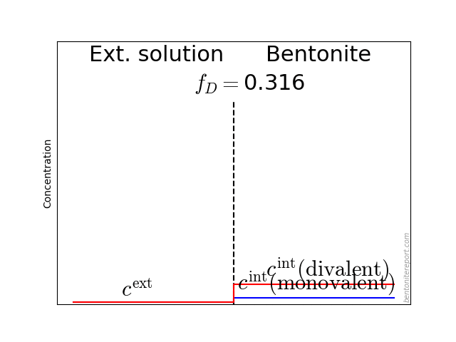
Consider an ordinary aqueous solution containing radioactive \(^{22}\mathrm{Na}\) and stable \(^{23}\mathrm{Na}\). The fraction of \(^{22}\mathrm{Na}\) ions can be written \(c_\mathrm{ext}/C_\mathrm{bkg}\), where \(c_\mathrm{ext}\) is the \(^{22}\mathrm{Na}\) concentration, and \(C_\mathrm{bkg}\) is the total sodium concentration (the “tracer” and “background” concentrations, respectively).

Since \(^{23}\mathrm{Na}\) and \(^{22}\mathrm{Na}\) are basically chemically indistinguishable, the same \(^{22}\mathrm{Na}\)-fraction will be maintained in any system with which this solution is in equilibrium. In particular, if the solution is in equilibrium with a montmorillonite interlayer solution, we can write

\begin{equation*} \frac{c_\mathrm{int}}{C_\mathrm{int}} = \frac{c_\mathrm{ext}}{C_\mathrm{bkg}} \tag{1} \end{equation*}

where \(c_\mathrm{int}\) and \(C_\mathrm{int}\) are the \(^{22}\mathrm{Na}\) and total interlayer concentrations, respectively. The total interlayer cation concentration (\(C_\mathrm{int}\)) can be handled in different ways, but it is important to note that this is a substantial number under all conditions, relating to the cation exchange capacity.⁵ Rearranging eq. 1 gives

\begin{equation*} c_\mathrm{int} = \frac{C_\mathrm{int}}{C_\mathrm{bkg}}\cdot c_\mathrm{ext} \end{equation*}

Since the interlayer cation concentration is always larger than the corresponding background concentration, the above equation tells us that the corresponding interlayer tracer concentration becomes enhanced, by the factor \(C_\mathrm{int}/C_\mathrm{bkg}\).

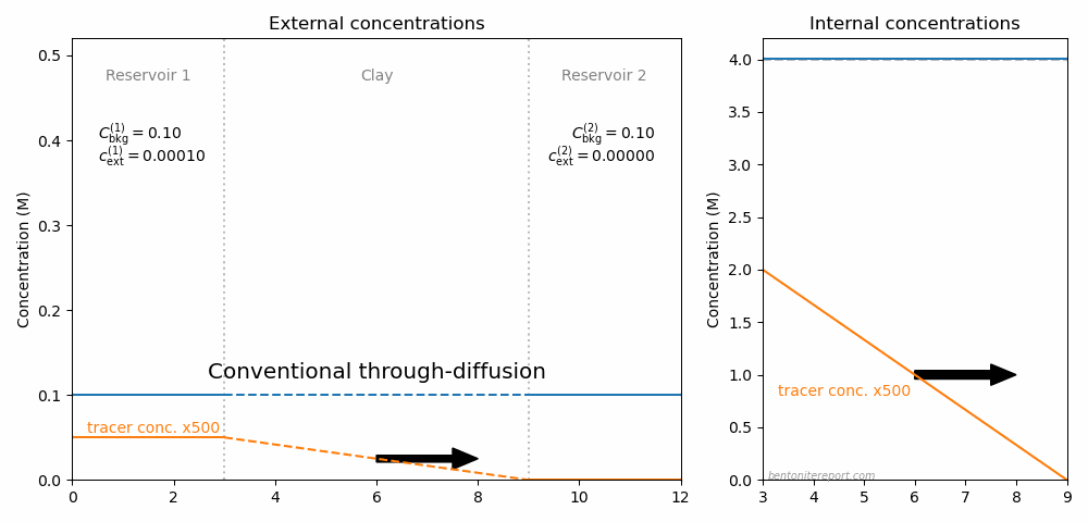
Conventional through-diffusion

This enhancement mechanism causes the diffusional behavior of \(^{22}\mathrm{Na}\) in conventional through-diffusion experiments in bentonite. In such experiments, the tracer concentration in the target reservoir is usually kept near zero, and the actual steady-state concentration gradient in the interlayers is

\begin{equation*} \frac{\partial c_\mathrm{int}}{\partial x} = \frac{0- C_\mathrm{int}/C_\mathrm{bkg}\cdot c_\mathrm{ext}^{(1)}} {L} = -\frac{C_\mathrm{int}}{C_\mathrm{bkg}}\cdot \frac{ c_\mathrm{ext}^{(1)} }{ L } \end{equation*}

where we have indexed the tracer concentration in the source reservoir with “\((1)\)”, labeled the sample length \(L\), and assumed that ions diffuse in the \(x\)-direction. The corresponding flux is thus (Fick’s law)

\begin{equation*} j_\mathrm{steady-state} = – \phi D_c\frac{\partial c_\mathrm{int}}{\partial x} = \phi D_c\cdot \frac{C_\mathrm{int}}{C_\mathrm{bkg}}\cdot \frac{c_\mathrm{ext}^{(1)} } {L} \tag{2} \end{equation*}

where \(D_c\) denotes the (macroscopic) diffusivity in the interlayers, and \(\phi\) is porosity. Keeping \(c_\mathrm{ext}^{(1)}\) constant, eq. 2 shows that the \(^{22}\mathrm{Na}\) steady-state flux increases indefinitely as the background concentration is made small, in full agreement with experimental observation.⁶

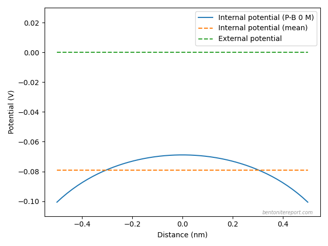
The picture below illustrates the concentration conditions in an conventional through-diffusion test.

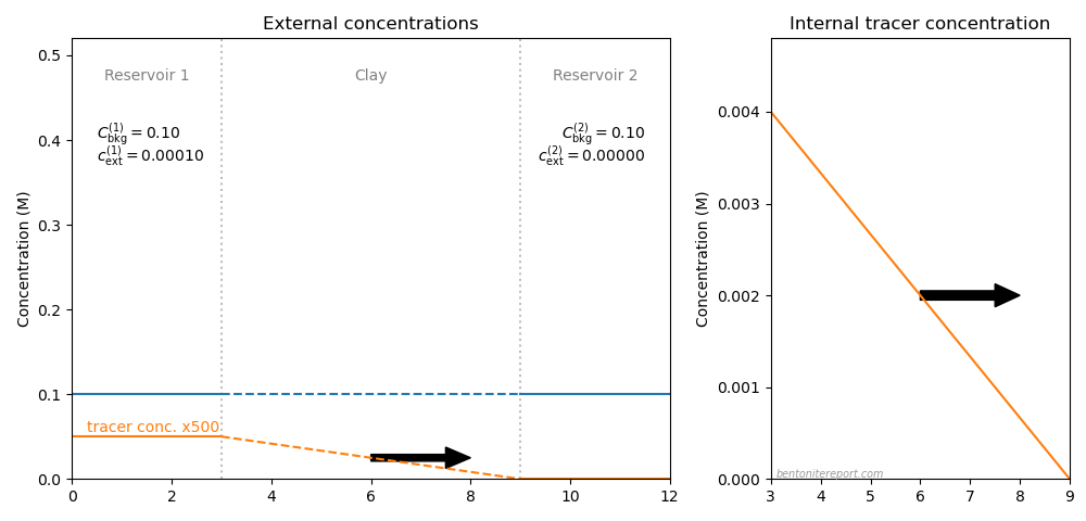
Here we have chosen \(C_\mathrm{int}=\) 4.0 M, the background concentration in the two reservoirs (blue) is put equal to 0.1 M, and the tracer concentration (orange) is put to 0.1 mM in reservoir 1 (and zero i reservoir 2). The corresponding internal tracer gradient is plotted in the right side diagram, and the resulting diffusive flux is indicated by the arrow.

“Uphill” diffusion

To explain the “uphill” effect the only modifications needed in the above derivation is to allow for different background concentrations in the external reservoirs, and to recognize that the tracer concentration in the clay on the “target” side (indexed “\((2)\)”) no longer is zero. Considering the tracer concentration enhancement at both interfaces, the steady-state interlayer concentration gradient then reads

\begin{equation*} \frac{\partial c_\mathrm{int}}{\partial x} = \frac{ C_\mathrm{int}/C_\mathrm{bkg}^{(2)}\cdot c_\mathrm{ext}^{(2)} -C_\mathrm{int}/C_\mathrm{bkg}^{(1)}\cdot c_\mathrm{ext}^{(1)}} {L} \end{equation*}

To be more concrete, let’s assume that \(C_\mathrm{bkg}^{(2)} = 5\cdot C_\mathrm{bkg}^{(1)}\), which is the same ratio as in Glaus et al. (2013). We then have

\begin{equation*} \frac{\partial c_\mathrm{int}}{\partial x} = \frac{C_\mathrm{int}}{C_\mathrm{bkg}^{(1)}} \cdot \frac{ c_\mathrm{ext}^{(2)}/5 – c_\mathrm{ext}^{(1)}} {L} \end{equation*}

giving the corresponding steady-state flux

\begin{equation*} j_\mathrm{steady-state} = \phi D_c\cdot \frac{C_\mathrm{int}}{C_\mathrm{bkg}^{(1)}} \cdot \frac{ c_\mathrm{ext}^{(1)} – c_\mathrm{ext}^{(2)}/5} {L} \end{equation*}

Note that we recover the conventional through-diffusion result (eq. 2) from this expression, if we put \(c_\mathrm{ext}^{(2)}= 0\). But if we e.g. set the tracer concentration equal in both reservoirs, we still have a flux from side \((1)\) to side \((2)\), of size \(j = 4/5 \cdot \phi D_c\cdot C_\mathrm{int}/C_\mathrm{bkg}^{(1)}\cdot c_\mathrm{ext}^{(1)}\). And even if we make \(c_\mathrm{ext}^{(2)}\) larger than \(c_\mathrm{ext}^{(1)}\) — as long as \(c_\mathrm{ext}^{(1)}< c_\mathrm{ext}^{(2)} < 5\cdot c_\mathrm{ext}^{(1)}\) — we still have a diffusive flux from side \((1)\) to side \((2)\), i.e seeming “uphill” diffusion.

Below is illustrated the concentration conditions in an “uphill” configuration.

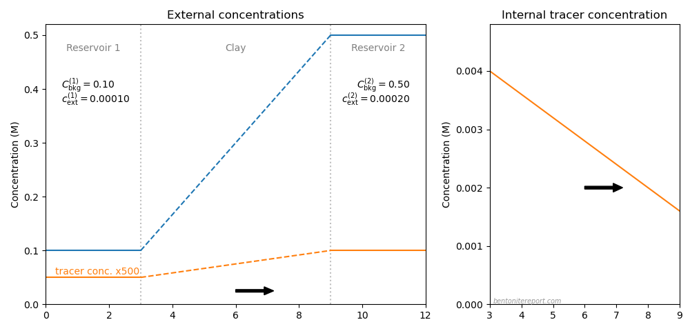
In contrast to the above illustration for conventional through-diffusion, the background concentration in reservoir 2 is here raised to 0.5 M and the tracer concentration in reservoir 2 is put equal to 0.2 mM. We see that, although tracers are transported to the reservoir with higher concentration, the process is still ordinary Fickian diffusion, as the internal tracer gradient has the same direction as in the conventional case.

We can now conclude what was stated above: The “uphill” diffusion effect is caused by exactly the same mechanism that cause the behavior of cation diffusion in conventional bentonite through-diffusion tests. This mechanism is ion equilibrium between clay and external solutions at the two interfaces. In this particular case, with sodium tracers diffusing in a sodium background, we don’t need to invoke the full ion equilibrium framework in order to quantify the fluxes, but can rely on the very robust result that any two systems in equilibrium have the same tracer fraction (eq. 1).

Reexamining the Tertre et al. (2024) statements

With the explanation for the “uphill” effect established, let’s re-examine the problematic statements in Tertre et al. (2024) identified above

Glaus et al. (2013) cannot be used to support a claim of “marked influence” of additional diffusional couplings. The opposite is true: Glaus et al. (2013) found no significant influence from mechanisms beyond those in chemically homogeneous conditions.
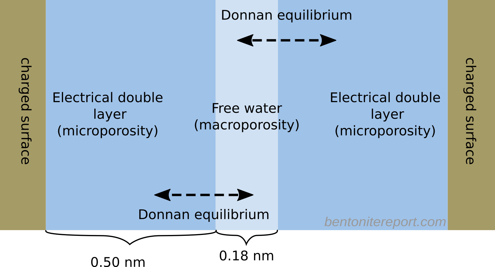
The “uphill” effect was predicted from taking the idea seriously that diffusion in compacted bentonite is fully governed by interlayer properties. Singling out Glaus et al. (2013) as the study that demonstrates the importance of diffuse layers⁷ therefore gives the wrong impression. Rather, what Glaus et al. (2013) demonstrates, in conjunction with corresponding conventional through-diffusion results, is that compacted bentonite contains insignificant amounts of bulk water (what Tertre et al. (2024) call “interparticle water”).

A way forward (if anybody cares)

After the uphill study was published I was for a while under the illusion that things would begin to change within the compacted bentonite research field. Not only did the study, to my mind, deal a fatal blow to any bentonite model that relies on the presence of a bulk water phase in the clay. It also opened up a whole new area of interesting studies to conduct. Now, some 11 years later, I can disappointingly conclude that not a single additional study has been presented that explore the ideas here discussed.⁸ And, regarding bentonite models, bulk water is apparently alive and kicking, as has been discussed ad nauseum on this blog.

Experimentally, there are a number of interesting questions looking for answers. In particular, we actually do expect additional mechanisms to play a role in chemically inhomogeneous systems, e.g. osmosis, and other effects due to presence of salt concentration gradients and electrostatic potential differences. It may be argued for why such effects are not significant in Glaus et al. (2013), but it is of course both of fundamental and practical interest to understand under which conditions they are. The original “uphill” study is e.g. performed at quite extreme density (\(1900\;\mathrm{m^3/kg}\)). How would the result differ at \(1600\;\mathrm{m^3/kg}\) or \(1300\;\mathrm{m^3/kg}\)? Also, how would the results change with other choices of the reservoir concentrations, and how would the results differ if one of the cations is not at trace level (e.g. a system with comparable amounts of sodium and potassium)?

Even under the conditions of the original study, there are several predictions left to verify. If e.g. \(c^{(1)}_\mathrm{ext} = c^{(2)}_\mathrm{ext}/5\), the theory predicts zero flux (implying \(D_e = 0\)). The theory also implies that when performing “conventional” through-diffusion, the actual level of the background concentration in the target reservoir is irrelevant, as long as the tracer concentration is kept at zero.

In fact, one can imagine making a whole cycle of through-diffusion tests to explore the ideas here discussed, as illustrated in this animation

The resulting steady-state flux for various external conditions is indicated by the arrow. Here, the full ion equilibrium framework was used to calculate the internal concentrations (giving an internal gradient also in \(C_\mathrm{int}\)). Background concentrations and total interlayer concentration is chosen to be comparable with Glaus et al. (2013), while the choice for tracer concentration is arbitrary.⁹

With the risk of sounding hubristic, the number of experiments suggested in the above animation could have given enough material for several Ph.D. theses. But here we are, in the year 2024, without even a replication of the “uphill” effect. Instead, a basically entire research field has been stuck for decades with the ludicrous idea that models of compacted bentonite should be based on a bulk water description. I find this both hilarious and horrific.

Footnotes

[1] For example (follow links to discussions on these issues):

It states the traditional diffusion-sorption model as being relevant in these systems. It is not.
It somehow manages to combine the traditional diffusion-sorption model with the effective porosity model for anion tracer diffusion, although these two models are incompatible.
Related to using the traditional diffusion-sorption model, it assumes \(D_e\) to be a real diffusion coefficient, which it is not. I find this particularly remarkable in a paper that deals with the presence of “saline gradients”. A motivation behind e.g. the “uphill” test is to point out the shortcomings of \(D_e\), as discussed in the rest of this blog post.
It claims that “anionic and cationic tracers do not experience the same overall accessible porosity”, which is unjustified.
It claims that “diffusion rates” of anions are decreased and “diffusion rates” of cations are increased, compared to “neutral species”, due to different interactions with diffuse layers. But this is not true generally.
It implicitly simply assumes a “stack”-view of these clay systems. But stacks don’t make much sense.

[2] I use the word “bentonite” here quite loosely. Tertre et al. (2024) use wordings such as “clayey samples”, “argillaceous rocks” and “clayey formation”, but it is clear that the presented material is supposed to apply to actual bentonite.

[3] I’m specifically thinking about that cation tracer through-diffusion tests at low background concentration is not a good idea, and that it is completely clear from the results presented in Tertre et al. (2024) that some of these are mainly controlled by diffusion in the confining filters. Estimating a “rock capacity factor” larger than 750 for sodium tracers in a sodium-clay (at 20 mM background concentration) should have set off all alarm bells.

[4] Regarding Soler et al. (2019), I think that whole study is problematic, which I might argue for in a separate blog post.

[5] Glaus et al. (2013) invoke the “exchange site” activity \([\mathrm{NaX}]\) to discuss this quantity. I personally prefer relating it to the quantity \(c_\mathrm{IL}\) that is defined within the homogeneous mixture model.

[6] This agreement has been shown to be quantitative, see e.g. Glaus et al. (2007), Birgersson and Karnland (2009) and Birgersson (2017). Note that this result is quite independent on how many “porosities” you choose to include in a model; it’s merely a consequence of treating the dominating pores (interlayers) adequately. Further, note that measuring the diverging fluxes in the limit of low background concentration becomes increasingly difficult, as the confining filters becomes rate limiting.

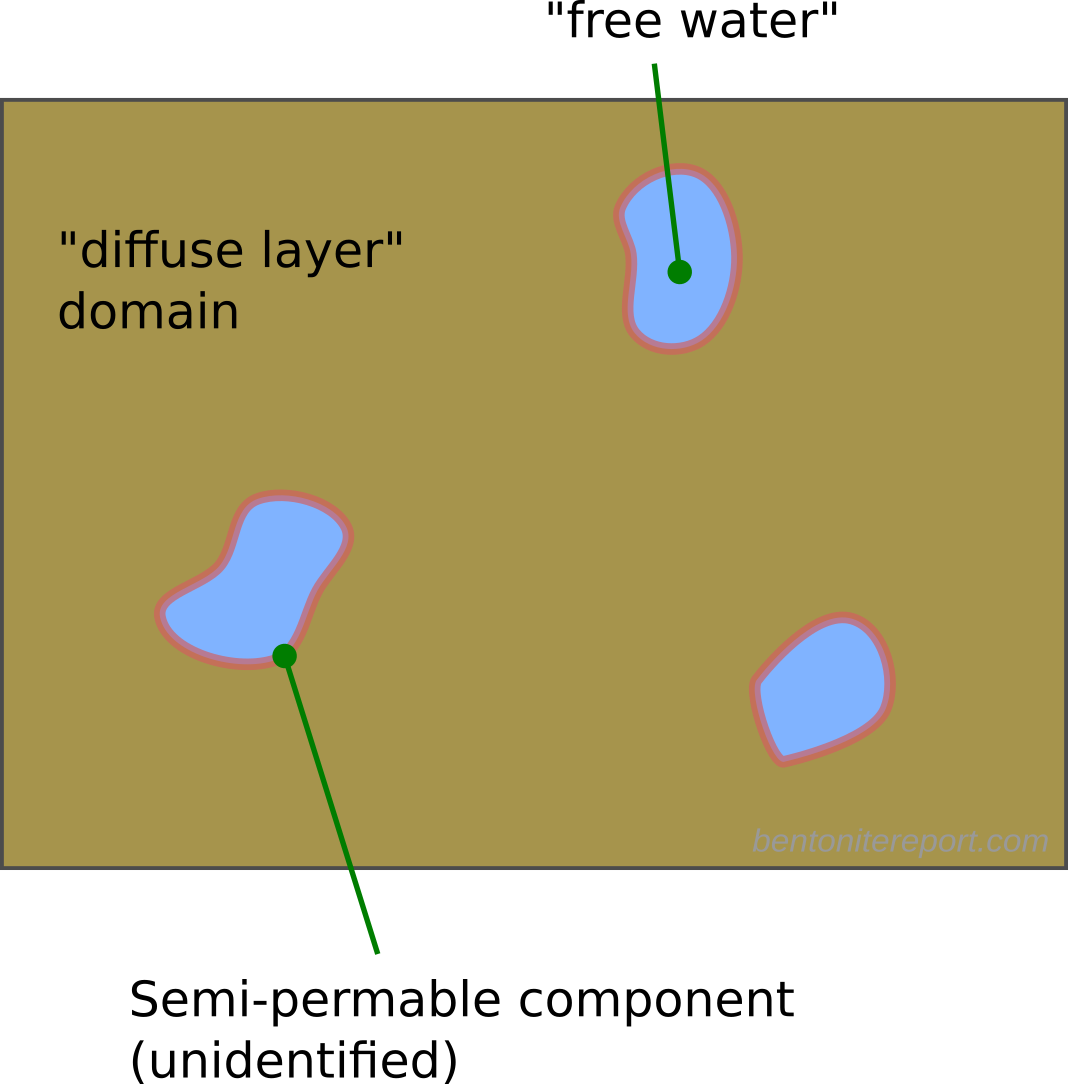
[7] In the present context, I presume the terms “diffuse layer” and “interlayer” to be more or less equivalent. Other authors instead make an unjustified distinction, that I have addressed here.

[8] There are a few examples of published studies where effects of the kind discussed here are present, but where the authors don’t seem to be aware of it.

[9] Tracer concentrations in Glaus et al. (2013) is much smaller, but this value does not affect any behavior, as long as it is small in comparison with total concentration.

Solving the Poisson-Boltzmann equation

1 Reply

To celebrate that I have built myself a tool for solving the Poisson-Boltzmann equation for two parallel charged plates and specified external solution, here is a cosy little animation

The animation shows the anion concentration profile (blue) between the plates as the distance varies, in systems in equilibrium with an external 100 mM 1:1 salt solution. Also plotted is the corresponding internal concentration level as calculated from the ideal Donnan equilibrium formula (orange). The layer charge density in the Poisson-Boltzmann calculation is 0.111 C/m², and the corresponding cation exchange capacity in the Donnan calculation is 0.891 eq/kg.

As the distance between the plates increases, the Poisson-Boltzmann profile increasingly deviates from the Donnan concentration. At lower density (larger plate distance) it is clear that the Poisson-Boltzmann solution allows for considerably more anions between the plates as compared with the Donnan result. On the other hand, for denser systems, the difference between the two solutions decreases; this is especially true when considering the relative difference — keep in mind that the external concentration is kept constant, at 100 mM.

In fact, in systems relevant for e.g. radioactive waste storage — spanning an effective montmorillonite density range from \(\rho_\mathrm{mmt} =\) 1.60 g/cm³ to \(\rho_\mathrm{mmt} =\) 1.15 g/cm³, say — the difference between the Poisson-Boltzmann and the Donnan results is virtually negligible (it should also be kept in mind that the continuum assumption underlying the Poisson-Boltzmann calculation is not valid in this density range). Here are plotted snapshots of these two limiting cases, together with the Poisson-Boltzmann solution for a single plate (the Gouy-Chapman model)

This figure clearly shows that the Gouy-Chapman model is not at all valid in any relevant system, unless you postulate larger voids in the bentonite. But why would you do that?

Multi-porosity models cannot be taken seriously (Semi-permeability, part II)

Leave a reply

“Multi-porosity” models¹ — i.e models that account for both a bulk water phase and one, or several, other domains within the clay — have become increasingly popular in bentonite research during the last couple of decades. These are obviously macroscopic, as is clear e.g. from the benchmark simulations described in Alt-Epping et al. (2015), which are specified to be discretized into 2 mm thick cells; each cell is consequently assumed to contain billions and billions individual montmorillonite particles. The macroscopic character is also relatively clear in their description of two numerical tools that have implemented multi-porosity

PHREEQC and CrunchFlowMC have implemented a Donnan approach to describe the electrical potential and species distribution in the EDL. This approach implies a uniform electrical potential \(\varphi^\mathrm{EDL}\) in the EDL and an instantaneous equilibrium distribution of species between the EDL and the free water (i.e., between the micro- and macroporosity, respectively). The assumption of instantaneous equilibrium implies that diffusion between micro- and macroporosity is not considered explicitly and that at all times the chemical potentials, \(\mu_i\), of the species are the same in the two porosities

On an abstract level, we may thus illustrate a multi-porosity approach something like this (here involving two domains)

The model is represented by one continuum for the “free water”/”macroporosity” and one for the “diffuse layer”/”microporosity”,² which are postulated to be in equilibrium within each macroscopic cell.

But such an equilibrium (Donnan equilibrium) requires a semi-permeable component. I am not aware of any suggestion for such a component in any publication on multi-porosity models. Likewise, the co-existence of diffuse layer and free water domains requires a mechanism that prevents swelling and maintains the pressure difference — also the water chemical potential should of course be the equal in the two “porosities”.³

Note that the questions of what constitutes the semi-permeable component and what prevents swelling have a clear answer in the homogeneous mixture model. This answer also corresponds to an easily identified real-world object: the metal filter (or similar component) separating the sample from the external solution. Multi-porosity models, on the other hand, attribute no particular significance to interfaces between sample and external solutions. Therefore, a candidate for the semi-permeable component has to be — but isn’t — sought elsewhere. Donnan equilibrium calculations are virtually meaningless without identifying this component.

The partitioning between diffuse layer and free water in multi-porosity models is, moreover, assumed to be controlled by water chemistry, usually by means of the Debye length. E.g. Alt-Epping et al. (2015) write

To determine the volume of the microporosity, the surface area of montmorillonite, and the Debye length, \(D_L\), which is the distance from the charged mineral surface to the point where electrical potential decays by a factor of e, needs to be known. The volume of the microporosity can then be calculated as \begin{equation*} \phi^\mathrm{EDL} = A_\mathrm{clay} D_L, \end{equation*} where \(A_\mathrm{clay}\) is the charged surface area of the clay mineral.

I cannot overstate how strange the multi-porosity description is. Leaving the abstract representation, here is an attempt to illustrate the implied clay structure, at the “macropore” scale

The view emerging from the above description is actually even more peculiar, as the “micro” and “macro” volume fractions are supposed to vary with the Debye length. A more general illustration of how the pore structure is supposed to function is shown in this animation (“I” denotes ionic strength)

What on earth could constitute such magic semi-permeable membranes?! (Note that they are also supposed to withstand the inevitable pressure difference.)

Here, the informed reader may object and point out that no researcher promoting multi-porosity has this magic pore structure in mind. Indeed, basically all multi-porosity publications instead vaguely claim that the domain separation occurs on the nanometer scale and present microscopic illustrations, like this (this is a simplified version of what is found in Alt-Epping et al. (2015))

In the remainder of this post I will discuss how the idea of a domain separation on the microscopic scale is even more preposterous than the magic membranes suggested above. We focus on three aspects:

The implied structure of the free water domain
The arbitrary domain division
Donnan equilibrium on the microscopic scale is not really a valid concept

Implied structure of the free water domain

I’m astonished by how little figures of the microscopic scale are explained in many publications. For instance, the illustration above clearly suggests that “free water” is an interface region with exactly the same surface area as the “double layer”. How can that make sense? Also, if the above structure is to be taken seriously it is crucial to specify the extensions of the various water layers. It is clear that the figure shows a microscopic view, as it depicts an actual diffuse layer.⁴ A diffuse layer width varies, say, in the range 1 – 100 nm,⁵ but authors seldom reveal if we are looking at a pore 1 nm wide or several hundred nm wide. Often we are not even shown a pore — the water film just ends in a void, as in the above figure.⁶

The vague nature of these descriptions indicates that they are merely “decorations”, providing a microscopic flavor to what in effect still is a macroscopic model formulation. In practice, most multi-porosity formulations provide some ad hoc mean to calculate the volume of the diffuse layer domain, while the free water porosity is either obtained by subtracting the diffuse layer porosity from total porosity, or by just specifying it. Alt-Epping et al. (2015), for example, simply specifies the “macroporosity”

The total porosity amounts to 47.6 % which is divided into 40.5 % microporosity (EDL) and 7.1 % macroporosity (free water). From the microporosity and the surface area of montmorillonite (Table 7), the Debye length of the EDL calculated from Eq. 11 is 4.97e-10 m.

Clearly, nothing in this description requires or suggests that the “micro” and “macroporosities” are adjacent waterfilms on the nm-scale. On the contrary, such an interpretation becomes quite grotesque, with the “macroporosity” corresponding to half a monolayer of water molecules! An illustration of an actual pore of this kind would look something like this

This interpretation becomes even more bizarre, considering that Alt-Epping et al. (2015) assume advection to occur only in this half-a-monolayer of water, and that the diffusivity is here a factor 1000 larger than in the “microporosity”.

As another example, Appelo and Wersin (2007) model a cylindrical sample of “Opalinus clay” of height 0.5 m and radius 0.1 m, with porosity 0.16, by discretizing the sample volume in 20 sections of width 0.025 m. The void volume of each section is consequently \(V_\mathrm{void} = 0.16\cdot\pi\cdot 0.1^2\cdot 0.025\;\mathrm{m^3} = 1.257\cdot10^{-4}\;\mathrm{m^3}\). Half of this volume (“0.062831853” liter) is specified directly in the input file as the volume of the free water;⁷ again, nothing suggests that this water should be distributed in thin films on the nm-scale. Yet, Appelo and Wersin (2007) provide a figure, with no length scale, similar in spirit to that above, that look very similar to this

They furthermore write about this figure (“Figure 2”)

It should be noted that the model can zoom in on the nm-scale suggested by Figure 2, but also uses it as the representative form for the cm-scale or larger.

I’m not sure I can make sense of this statement, but it seems that they imply that the illustration can serve both as an actual microscopic representation of two spatially separated domains and as a representation of two abstract continua on the macroscopic scale. But this is not true!

Interpreted macroscopically, the vertical dimension is fictitious, and the two continua are in equilibrium in each paired cell. On a microscopic scale, on the other hand, equilibrium between paired cells cannot be assumed a priori, and it becomes crucial to specify both the vertical and horizontal length scales. As Appelo and Wersin (2007) formulate their model assuming equilibrium between paired cells, it is clear that the above figure must be interpreted macroscopically (the only reference to a vertical length scale is that the “free solution” is located “at infinite distance” from the surface).

We can again work out the implications of anyway interpreting the model microscopically. Each clay cell is specified to contain a surface area of \(A_\mathrm{surf}=10^5\;\mathrm{m^2}\).⁸ Assuming a planar geometry, the average pore width is given by (\(\phi\) denotes porosity and \(V_\mathrm{cell}\) total cell volume)

\begin{equation} d = 2\cdot \phi \cdot \frac{V_\mathrm{cell}}{A_\mathrm{surf}} = 2\cdot \frac{V_\mathrm{void}}{A_\mathrm{surf}} = 2\cdot \frac{1.26\cdot 10^{-4}\;\mathrm{m^3}}{10^{5}\;\mathrm{m^2}} = 2.51\;\mathrm{nm} \end{equation}

The double layer thickness is furthermore specified to be 0.628 nm.⁹ A microscopic interpretation of this particular model thus implies that the sample contains a single type of pore (2.51 nm wide) in which the free water is distributed in a thin film of width 1.25 nm — i.e. approximately four molecular layers of water!

Rather than affirming that multi-porosity model formulations are macroscopic at heart, parts of the bentonite research community have instead doubled down on the confusing idea of having free water distributed on the nm-scale. Tournassat and Steefel (2019) suggest dealing with the case of two parallel charged surfaces in terms of a “Dual Continuum” approach, providing a figure similar to this (surface charge is -0.11 C/m² and external solution is 0.1 M of a 1:1 electrolyte)

Note that here the perpendicular length scale is specified, and that it is clear from the start that the electrostatic potential is non-zero everywhere. Yet, Tournassat and Steefel (2019) mean that it is a good idea to treat this system as if it contained a 0.7 nm wide bulk water slice at the center of the pore. They furthermore express an almost “postmodern” attitude towards modeling, writing

It should be also noted here that this model refinement does not imply necessarily that an electroneutral bulk water is present at the center of the pore in reality. This can be appreciated in Figure 6, which shows that the Poisson–Boltzmann predicts an overlap of the diffuse layers bordering the two neighboring surfaces, while the dual continuum model divides the same system into a bulk and a diffuse layer water volume in order to obtain an average concentration in the pore that is consistent with the Poisson–Boltzmann model prediction. Consequently, the pore space subdivision into free and DL water must be seen as a convenient representation that makes it possible to calculate accurately the average concentrations of ions, but it must not be taken as evidence of the effective presence of bulk water in a nanoporous medium.

I can only interpret this way of writing (“…does not imply necessarily that…”, “…must not be taken as evidence of…”) that they mean that in some cases the bulk phase should be interpreted literally, while in other cases the bulk phase should be interpreted just as some auxiliary component. It is my strong opinion that such an attitude towards modeling only contributes negatively to process understanding (we may e.g. note that later in the article, Tournassat and Steefel (2019) assume this perhaps non-existent bulk water to be solely responsible for advective flow…).

I say it again: no matter how much researchers discuss them in microscopic terms, these models are just macroscopic formulations. Using the terminology of Tournassat and Steefel (2019), they are, at the end of the day, represented as dual continua assumed to be in local equilibrium (in accordance with the first figure of this post). And while researchers put much effort in trying to give these models a microscopic appearance, I am not aware of anyone suggesting a reasonable candidate for what actually could constitute the semi-permeable component necessary for maintaining such an equilibrium.

Arbitrary division between diffuse layer and free water

Another peculiarity in the multi-porosity descriptions showing that they cannot be interpreted microscopically is the arbitrary positioning of the separation between diffuse layer and free water. We saw earlier that Alt-Epping et al. (2015) set this separation at one Debye length from the surface, where the electrostatic potential is claimed to have decayed by a factor of e. What motivates this choice?

Most publications on multi-porosity models define free water as a region where the solution is charge neutral, i.e. where the electrostatic potential is vanishingly small.¹⁰ At the point chosen by Alt-Epping et al. (2015), the potential is about 37% of its value at the surface. This cannot be considered vanishingly small under any circumstance, and the region considered as free water is consequently not charge neutral.

The diffuse layer thickness chosen by Appelo and Wersin (2007) instead corresponds to 1.27 Debye lengths. At this position the potential is about 28% of its value at the surface, which neither can be considered vanishingly small. At the mid point of the pore (1.25 nm), the potential is about 8%¹¹ of the value at the surface (corresponding to about 2.5 Debye lengths). I find it hard to accept even this value as vanishingly small.

Note that if the boundary distance used by Appelo and Wersin (2007) (1.27 Debye lengths) was used in the benchmark of Alt-Epping et al. (2015), the diffuse layer volume becomes larger than the total pore volume! In fact, this occurs in all models of this kind for low enough ionic strength, as the Debye length diverges in this limit. Therefore, many multi-porosity model formulations include clunky “if-then-else” clauses,¹² where the system is treated conceptually different depending on whether or not the (arbitrarily chosen) diffuse layer domain fills the entire pore volume.¹³

In the example from Tournassat and Steefel (2019) the extension of the diffuse layer is 1.6 nm, corresponding to about 1.69 Debye lengths. The potential is here about 19% of the surface value (the value in the midpoint is 12% of the surface value). Tournassat and Appelo (2011) uses yet another separation distance — two Debye lengths — based on misusing the concept of exclusion volume in the Gouy-Chapman model.

With these examples, I am not trying to say that a better criterion is needed for the partitioning between diffuse layer and bulk. Rather, these examples show that such a partitioning is quite arbitrary on a microscopic scale. Of course, choosing points where the electrostatic potential is significant makes no sense, but even for points that could be considered having zero potential, what would be the criterion? Is two Debye lengths enough? Or perhaps four? Why?

These examples also demonstrate that researchers ultimately do not have a microscopic view in mind. Rather, the “microscopic” specifications are subject to the macroscopic constraints. Alt-Epping et al. (2015), for example, specifies a priori that the system contains about 15% free water, from which it follows that the diffuse layer thickness must be set to about one Debye length (given the adopted surface area). Likewise, Appelo and Wersin (2007) assume from the start that Opalinus clay contains 50% free water, and set up their model accordingly.¹⁴ Tournassat and Steefel (2019) acknowledge their approach to only be a “convenient representation”, and don’t even relate the diffuse layer extension to a specific value of the electrostatic potential.¹⁵ Why the free water domain anyway is considered to be positioned in the center of the nanopore is a mystery to me (well, I guess because sometimes this interpretation is supposed to be taken literally…).

Note that none of the free water domains in the considered models are actually charged, even though the electrostatic potential in the microscopic interpretations is implied to be non-zero. This just confirms that such interpretations are not valid, and that the actual model handling is the equilibration of two (or more) macroscopic, abstract, continua. The diffuse layer domain is defined by following some arbitrary procedure that involves microscopic concepts. But just because the diffuse layer domain is quantified by multiplying a surface area by some multiple of the Debye length does not make it a microscopic entity.⁴

Donnan effect on the microscopic scale?!

Although we have already seen that we cannot interpret multi-porosity models microscopically, we have not yet considered the weirdest description adopted by basically all proponents of these models: they claim to perform Donnan equilibrium calculations between diffuse layer and free water regions on the microscopic scale!

The underlying mechanism for a Donnan effect is the establishment of charge separation, which obviously occur on the scale of the ions, i.e. on the microscopic scale. Indeed, a diffuse layer is the manifestation of this charge separation. Donnan equilibrium can consequently not be established within a diffuse layer region, and discontinuous electrostatic potentials only have meaning in a macroscopic context.

Consider e.g. the interface between bentonite and an external solution in the homogeneous mixture model. Although this model ignores the microscopic scale, it implies charge separation and a continuously varying potential on this scale, as illustrated here

The regions where the potential varies are exactly what we categorize as diffuse layers (exemplified in two ideal microscopic geometries).

The discontinuous potentials encountered in multi-porosity model descriptions (see e.g. the above “Dual Continuum” potential that varies discontinuously on the angstrom scale) can be drawn on paper, but don’t convey any physical meaning.

Here I am not saying that Donnan equilibrium calculations cannot be performed in multi-porosity models. Rather, this is yet another aspect showing that such models only have meaning macroscopically, even though they are persistently presented as if they somehow consider the microscopic scale.

An example of this confusion of scales is found in Alt-Epping et al. (2018), who revisit the benchmark problem of Alt-Epping et al. (2015) using an alternative approach to Donnan equilibrium: rather than directly calculating the equilibrium, they model the clay charge as immobile mono-valent anions, and utilize the Nernst-Planck equations. They present “the conceptual model” in a figure very similar to this one

This illustration simultaneously conveys both a micro- and macroscopic view. For example, a mineral surface is indicated at the bottom, suggesting that we supposedly are looking at an actual interface region, in similarity with the figures we have looked at earlier. Moreover, the figure contains entities that must be interpreted as individual ions, including the immobile “clay-anions”. As in several of the previous examples, no length scale is provided (neither perpendicular to, nor along the “surface”).

On the other hand, the region is divided into cells, similar to the illustration in Appelo and Wersin (2007). These can hardly have any other meaning than to indicate the macroscopic discretization in the adopted transport code (FLOTRAN). Also, as the “Donnan porosity” region contains the “clay-anions” it can certainly not represent a diffuse layer extending from a clay surface; the only way to make sense of such an “immobile-anion” solution is that it represents a macroscopic homogenized clay domain (a homogeneous mixture!).

Furthermore, if the figure is supposed to show the microscopic scale there is no Donnan effect, because there is no charge separation! Taking the depiction of individual ions seriously, the interface region should rather look something like this in equilibrium

This illustrates the fundamental problem with a Donnan effect between microscopic compartments: the effect requires a charge separation, whose extension is the same as the size of the compartments assumed to be in equilibrium.¹⁶

Despite the confusion of the illustration in Alt-Epping et al. (2018), it is clear that a macroscopic model is adopted, as in our previous examples. In this case, the model is explicitly 2-dimensional, and the authors utilize the “trick” to make diffusion much faster in the perpendicular direction compared to the direction along the “surface”. This is achieved either by making the perpendicular diffusivity very high, or by making the perpendicular extension small. In any case, a perpendicular length scale must have been specified in the model, even if it is nowhere stated in the article. The same “trick” for emulating Donnan equilibrium is also used by Jenni et al. (2017), who write

In the present model set-up, this approach was implemented as two connected domains in the z dimension: one containing all minerals plus the free porosity (z=1) and the other containing the Donnan porosity, including the immobile anions (CEC, z=2, Fig. 2). Reproducing instantaneous equilibrium between Donnan and free porosities requires a much faster diffusion between the porosity domains than along the porosity domains.

Note that although the perpendicular dimension (\(z\)) here is referred to without unit(!), this representation only makes sense in a macroscopic context.

Jenni et al. (2017) also provide a statement that I think fairly well sums up the multi-porosity modeling endeavor:¹⁷

In a Donnan porosity concept, cation exchange can be seen as resulting from Donnan equilibrium between the Donnan porosity and the free porosity, possibly moderated by additional specific sorption. In CrunchflowMC or PhreeqC (Appelo and Wersin, 2007; Steefel, 2009; Tournassat and Appelo, 2011; Alt-Epping et al., 2014; Tournassat and Steefel, 2015), this is implemented by an explicit partitioning function that distributes aqueous species between the two pore compartments. Alternatively, this ion partitioning can be modelled implicitly by diffusion and electrochemical migration (Fick’s first law and Nernst-Planck equations) between the free porosity and the Donnan porosity, the latter containing immobile anions representing the CEC. The resulting ion compositions of the two equilibrated porosities agree with the concentrations predicted by the Donnan equilibrium, which can be shown in case studies (unpublished results, Gimmi and Alt-Epping).

Ultimately, these are models that, using one approach or the other, simply calculates Donnan equilibrium between two abstract, macroscopically defined domains (“porosities”, “continua”). Microscopic interpretations of these models lead — as we have demonstrated — to multiple absurdities and errors. I am not aware of any multi-porosity approach that has provided any kind of suggestion for what constitutes the semi-permeable component required for maintaining the equilibrium they are supposed to describe. Alternatively expressed: what, in the previous figure, prevents the “immobile anions” from occupying the entire clay volume?

The most favorable interpretation I can make of multi-porosity approaches to bentonite modeling is a dynamically varying “macroporosity”, involving magical membranes (shown above). This, in itself, answers why I cannot take multi-porosity models seriously. And then we haven’t yet mentioned the flawed treatment of diffusive flux.

Semi-permeability, part I

Footnotes

[1] This category has many other names, e.g. “dual porosity” and “dual continuum”, models. Here, I mostly use the term “multi-porosity” to refer to any model of this kind.

[2] These compartments have many names in different publications. The “diffuse layer” domain is also called e.g. “electrical double layer (EDL)”, “diffuse double layer (DDL)”, “microporosity”, or “Donnan porosity”, and the “free water” is also called e.g. “macroporosity”, “bulk water”, “charge-free” (!), or “charge-neutral” porewater. Here I will mostly stick to using the terms “diffuse layer” and “free water”.

[3] This lack of a full description is very much related to the incomplete description of so-called “stacks” — I am not aware of any reasonable suggestion of a mechanism for keeping stacks together.

[4] Note the difference between a diffuse layer and a diffuse layer domain. The former is a structure on the nm-scale; the latter is a macroscopic, abstract model component (a continuum).

[5] The scale of an electric double layer is set by the Debye length, \(\kappa^{-1}\). From the formula for a 1:1 electrolyte, \(\kappa^{-1} = 0.3 \;\mathrm{nm}/\sqrt{I}\), the Debye length is seen to vary between 0.3 nm and 30 nm when ionic strength is varied between 1.0 M to 0.0001 M (\(I\) is the numerical value of the ionic strength expressed in molar units). Independent of the value of the factor used to multiply \(\kappa^{-1}\) in order to estimate the double layer extension, I’d say that the estimation 1 – 100 nm is quite reasonable.

[6] Here, the informed reader may perhaps point out that authors don’t really mean that the free water film has exactly the same geometry as the diffuse layer, and that figures like the one above are more abstract representations of a more complex structure. Figures of more complex pore structures are actually found in many multi-porosity papers. But if it is the case that the free water part is not supposed to be interpreted on the microscopic scale, we are basically back to a magic membrane picture of the structure! Moreover, if the free water is not supposed to be on the microscopic scale, the diffuse layer will always have a negligible volume, and these illustrations don’t provide a mean for calculating the partitioning between “micro” and “macroporosity”.

It seems to me that not specifying the extension of the free water is a way for authors to dodge the question of how it is actually distributed (and, as a consequence, to not state what constitutes the semi-permeable component).

[7] The PHREEQC input files are provided as supplementary material to Appelo and Wersin (2007). Here I consider the input corresponding to figure 3c in the article. The free water is specified with keyword “SOLUTION”.

[8] Keyword “SURFACE” in the PHREEQC input file for figure 3c in the paper.

[9] Using the identifier “-donnan” for the “SURFACE” keyword.

[10] We assume a boundary condition such that the potential is zero in the solution infinitely far away from any clay component.

[11] Assuming exponential decay, which is only strictly true for a single clay layer of low charge.

[12] For example, Tournassat and Steefel (2019) write (\(f_{DL}\) denotes the volume fraction of the diffuse layer):

In PHREEQC and CrunchClay, the volume of the diffuse layer (\(V_{DL}\) in m³), and hence the \(f_{DL}\) value, can be defined as a multiple of the Debye length in order to capture this effect of ionic strength on \(f_{DL}\): \begin{equation*} V_{DL} = \alpha_{DL}\kappa^{-1}S \tag{22} \end{equation*} \begin{equation*} f_{DL} = V_{DL}/V_{pore} \end{equation*} […] it is obvious that \(f_{DL}\) cannot exceed 1. Equation (22) must then be seen as an approximation, the validity of which may be limited to small variations of ionic strength compared to the conditions at which \(f_{DL}\) is determined experimentally. This can be appreciated by looking at the results obtained with a simple model where: \begin{equation*} \alpha_{DL} = 2\;\mathrm{if}\;4\kappa^{-1} \le V_{pore}/S\;\mathrm{and,} \end{equation*} \begin{equation*} f_{DL} = 1 \;\mathrm{otherwise.} \end{equation*}

[13] Some tools (e.g. PHREEQC) allow to put a maximum size limit on the diffuse layer domain, independent of chemical conditions. This is of course only a way for the code to “work” under all conditions.

[14] As icing on the cake, these estimations of free water in bentonite (15%) and Opalinus clay (50%) appear to be based on the incorrect assumption that “anions” only reside in such compartments. In the present context, this handling is particularly confusing, as a main point with multi-porosity models (I assume?) is to evaluate ion concentrations in other types of compartments.

[15] Yet, Tournassat and Steefel (2019) sometimes seem to favor the choice of two Debye lengths (see footnote 12), for unclear reasons.

[16] Donnan equilibrium between microscopic compartments can be studied in molecular dynamics simulations, but they require the considered system to be large enough for the electrostatic potential to reach zero. The semi-permeable component in such simulations is implemented by simply imposing constraints on the atoms making up the clay layer.

[17] I believe the referred unpublished results now are published: Gimmi and Alt-Epping (2018).

How salt equilibrium concentrations may be overestimated

1 Reply

Saturating with saline solution

When discussing semi-permeability, we noted that a bentonite sample that is saturated with a saline solution probably contains more salt in the initial stages of the process than what is dictated by the final state Donnan equilibrium. This salt must consequently diffuse out of the sample before equilibrium is reached.

The reason for such a possible “overshoot” of the clay concentration is that an infiltrating solution is not subject to a Donnan effect (between sample and external solution) when it fills out the air-filled voids of an unsaturated sample. Also, even if the region near the interface to the external solution becomes saturated — so that a Donnan effect is active — a sample may still take up more salt than prescribed by the final state, due to hyperfiltration: with a net inflow of water and an active Donnan effect, salt will accumulate at the inlet interface (unless the interface is flushed). This increased concentration, in turn, alters the Donnan equilibrium at the interface, with the effect that more salt diffuses into the clay.

These effects are relevant for our ongoing assessment of studies of chloride equilibrium concentrations. If bentonite samples are saturated with saline solutions, without taking precautions against these effects, evaluated equilibrium concentrations may be overestimated. Note that, even if saturating a sample may be relatively fast, it may take a long time for salt to reach full equilibrium, depending on details of the experimental set-up. In particular, if the set-up is such that the external solution does not flow past the inlet, equilibration may take a very long time, being limited by diffusion in filters and tubing.

Interface excess salt

Another way for evaluated salt concentrations to overestimate the true equilibrium value — which is independent of whether or not the sample has been saturated with a saline solution — is due to excess salt at the sample interfaces.

Suppose that you determine the equilibrium salt concentration in a bentonite sample in the following way. First you prepare the sample in a test cell and contact it with an external salt solution via filters. When the system (bentonite + solution) has reached equilibrium (taking all the precautions against overestimation discussed above), the concentration profile may be conceptualized like this

The aim is to determine \(\bar{c}_\mathrm{clay}\), the clay concentration of the species of interest (e.g. chloride), and to relate it to the corresponding concentration in the external solution (\(c_ \mathrm{ext}\)).

After ensuring the value of \(c_\mathrm{ext}\) (e.g. by sampling or controlling the external solution), you unload the test cell and isolate the bentonite sample. In doing so, we must keep in mind that the sample will begin to swell as soon as the force on it is released, if only water is available. In the present example it is difficult not to imagine that some water is available, e.g. in the filters.¹

It is thus plausible that the actual concentration profile look something like this directly after the sample has been isolated

We will refer to the elevated concentration at the interfaces as the interface excess. The exact shape of the resulting concentration profile depends reasonably on the detailed procedure for isolating the sample.² If the ion content of the sample is measured as a whole, and/or if the sample is stored for an appreciable amount of time before further analysis (so that the profile evens out due to diffusion), it is clear that the evaluated ion content will be larger than the actual clay concentration.

To quantify how much the clay concentration may be overestimated due to the interface excess, we introduce an effective penetration depth, \(\delta\)

\(\delta\) corresponds to a depth of the external concentration that gives the same interface excess as the actual distribution. Using this parameter, it is easy to see that the clay concentration evaluated as the average over the entire sample is

\begin{equation} \bar{c}_\mathrm{eval} = \bar{c}_\mathrm{clay}+\frac{2\cdot\delta} {L} \cdot \left (c_\mathrm{ext} – \bar{c}_\mathrm{clay} \right ) \end{equation}

By dividing by the actual value \(\bar{c}_\mathrm{clay}\), we get an expression for the relative overestimation

\begin{equation} \frac{\bar{c}_\mathrm{eval}}{\bar{c}_\mathrm{clay}} = 1 + \frac{2\cdot\delta} {L} \cdot \left (\frac{c_\mathrm{ext}}{\bar{c}_\mathrm{clay}} – 1 \right ) \tag{1} \end{equation}

This expression is quite interesting. We see that the relative overestimation, reasonably, depends linearly on \(\delta\) and on the inverse of sample length. But the expression also contains the ratio \(r \equiv c_\mathrm{ext}/\bar{c}_\mathrm{clay}\), indicating that the effect may be more severe for systems where the clay concentration is small in comparison to the external concentration (high density, low \(c_\mathrm{ext}\)).

An interface excess is more than a theoretical concept, and is frequently observed e.g. in anion through-diffusion studies. We have previously encountered them when assessing the diffusion studies of Muurinen et al. (1988) and Molera et al. (2003).³ Van Loon et al. (2007) clearly demonstrate the phenomenon, as they evaluate the distribution of stable chloride (the background electrolyte) in the samples after performing the diffusion tests.⁴ Here is an example of the chloride distribution in a sample of density 1.6 g/cm³ and background concentration of 0.1 M⁵

The line labeled \(\bar{c}_\mathrm{clay}\) is evaluated from the average of only the interior sections (0.0066 M), while the line labeled \(\bar{c}_\mathrm{eval}\) is the average of all sections (0.0104 M). Using the full sample to evaluate the chloride clay concentration thus overestimates the value by a factor 1.6. From eq. 1, we see that this corresponds to \(\delta = 0.2\) mm. For a sample of length 5 mm with the same penetration depth, the corresponding overestimation is a factor of 2.1.

Here is plotted the relative overestimation (eq. 1) as a function of \(\delta\) for several systems of varying length and \(r\) (\(= c^\mathrm{ext}/\bar{c}_\mathrm{clay}\))

We see that systems with large \(r\) and/or small \(L\) become hypersensitive to this effect. Thus, even if it may be expected that \(\delta\) decreases with increasing \(r\)⁶, we may still expect an increased overestimation for such systems.

To avoid this potential overestimation of the clay concentration, I guess the best practice is to quickly remove the first couple of millimeters on both sides of a sample after it has been unloaded. In many through-diffusion tests, this is done as part of the study, as the concentration profile across the sample often is measured. In studies where samples are merely equilibrated with an external solution, however, removing the interface regions may not be considered.

Summary

We have here discussed some plausible reasons for why an evaluated equilibrium salt concentration in a clay sample may be overestimated:

If samples are saturated directly with a saline solution. Better practice is to first saturate the sample with pure water (or a dilute solution) and then to equilibrate with respect to salt in a second stage.
If the external solution is not circulated. Diffusion may then occur over very long distances (depending on test design). The reasonable practice is to always circulate external solutions.
If interface excess is not handled. This is an issue even if saturation is done with pure water. The most convenient way to deal with this is to section off the first millimeters on both sides of the samples as quickly as possible after they are unloaded.

Footnotes

[1] One way to minimize this possible effect could be to empty the filter before unloading the test cell. This may, however, be difficult unless the filter itself is flushable. Also, you may run into the problem of beginning to dry the sample.

[2] The only study I’m aware of that has systematically investigated these types of concentration profiles is Glaus et al. (2011). They claim, if I understand correctly, that the interface excess is not caused by swelling during dismantling. Rather, they mean that the profile is the result of an intrinsic density decrease that occurs in interface regions. Still, they don’t discuss how swelling are supposed to be inhibited, neither during dismantling, nor in order for the density inhomogeneity to remain. Under any circumstance, the conclusions in this blog post are not dependent on the cause for the presence of a salt interface excess.

[3] In through-diffusion tests, the problem of the interface excess is usually not that the equilibrium clay concentration is systematically overestimated, since the detailed concentration profile often is sampled in the final state. Instead, the problem becomes how to separate the linear and non-linear parts of the profile.

[4] Van Loon et al. (2007) will be assessed regarding evaluated chloride equilibrium concentrations in a future blog post. However, the study was considered in the post on the failure of Archie’s law in bentonite. Update (220721): Van Loon et al. (2007) is assessed in detail here.

[5] Van Loon et al. (2007) reports evaluated values of “effective porosity”, \(\epsilon_\mathrm{eff}\). I have calculated the clay concentration from these as \(\bar{c}_\mathrm{clay} = c_\mathrm{ext}\cdot \epsilon_\mathrm{eff}/\phi\), where \(\phi\) is the physical porosity. Note that \(\bar{c}_\mathrm{clay}\) is a model independent parameter, while \(\epsilon_\mathrm{eff}\) certainly is not.

[6] Because \(r\) and \(\delta\) may co-vary with density.

Semi-permeability, part I

Leave a reply

Descriptions in bentonite literature

What do authors mean when they say that bentonite has semi-permeable properties? Take for example this statement, from Bradbury and Baeyens (2003)¹

[…] highly compacted bentonite can function as an efficient semi-permeable membrane (Horseman et al., 1996). This implies that the re-saturation of compacted bentonite involves predominantly the movement of water molecules and not solute molecules.

Judging from the reference to Horseman et al. (1996) — which we look at below — it is relatively clear that Bradbury and Baeyens (2003) allude to the concept of salt exclusion when speaking of “semi-permeability” (although writing “solute molecules”). But a lowered equilibrium salt concentration does not automatically say that salt is less transferable.

A crucial question is what the salt is supposed to permeate. Note that a semi-permeable component is required for defining both swelling pressure and salt exclusion. In case of bentonite, this component is impermeable to the clay particles, while it is fully permeable to ions and water (in a lab setting, it is typically a metal filter). But Bradbury and Baeyens (2003) seem to mean that in the process of transferring aqueous species between an external reservoir and bentonite, salt is somehow effectively hindered to be transferred. This does not make much sense.

Consider e.g. the process mentioned in the quotation, i.e. to saturate a bentonite sample with a salt solution. With unsaturated bentonite, most bets are off regarding Donnan equilibrium, and how salt is transferred depends on the details of the saturation procedure; we only know that the external and internal salt concentrations should comply with the rules for salt exclusion once the process is finalized.

Imagine, for instance, an unsaturated sample containing bentonite pellets on the cm-scale that very quickly is flushed with the saturating solution, as illustrated in this state-of-the-art, cutting-edge animation

The evolution of the salt concentration in the sample will look something like this

Initially, as the saturating solution flushes the sample, the concentration will be similar to that of the external concentration (\(c_\mathrm{ext}\)). As the sample reaches saturation, it contains more salt than what is dictated by Donnan equilibrium (\(c_\mathrm{eq.}\)), and salt will diffuse out.

In a process like this it should be obvious that the bentonite not in any way is effectively impermeable to the salt. Note also that, although this example is somewhat extreme, the equilibrium salt concentration is probably reached “from above” in most processes where the clay is saturated with a saline solution: too much salt initially enters the sample (when a “microstructure” actually exists) and is later expelled.

Also for mass transfer between an external solution and an already saturated sample does it not make sense to speak of “semi-permeability” in the way here discussed. Consider e.g. a bentonite sample initially in equilibrium with an external 0.3 M NaCl solution, where the solution suddenly is switched to 1.0 M. Salt will then start to diffuse into the sample until a new (Donnan) equilibrium state is reached. Simultaneously (a minute amount of) water is transported out of the clay, in order for the sample to adapt to the new equilibrium pressure.²

There is nothing very “semi-permeabilic” going on here — NaCl is obviously free to pass into the clay. That the equilibrium clay concentration in the final state happens to be lower than in the external concentration is irrelevant for how how difficult it is to transfer the salt.

But it seems that many authors somehow equate “semi-permeability” with salt exclusion, and also mean that this “semi-permeability” is caused by reduced mobility for ions within the clay. E.g. Horseman et al. (1996) write (in a section entitled “Clays as semi-permeable membranes”)

[…] the net negative electrical potential between closely spaced clay particles repel anions attempting to migrate through the narrow aqueous films of a compact clay, a phenomenon known as negative adsorption or Donnan exclusion. In order to maintain electrical neutrality in the external solution, cations will tend to remain with their counter-ions and their movement through the clay will also be restricted (Fritz, 1986). The overall effect is that charged chemical species do not move readily through a compact clay and neutral water molecules may be able to pass more freely.

It must be remembered that Donnan exclusion occurs in many systems other than “compact clay”. By instead considering e.g. a ferrocyanide solution, it becomes clear that salt exclusion has nothing to do with how hindered the ions are to move in the system (as long as they move). KCl is, of course, not excluded from a potassium ferrocyanide system because ferrocyanide repels chloride, nor does such interactions imply restricted mobility (repulsion occurs in all salt solutions). Similarly, salt is not excluded from bentonite because of repulsion between anions and surfaces (also, a negative potential does not repel anything — charge does).

In the above quotation it is easy to spot the flaw in the argument by switching roles of anions and cations; you may equally incorrectly say that cations are attracted, and that anions tag along in order to maintain charge neutrality.

The idea that “semi-permeability” (and “anion” exclusion) is caused by mobility restrictions for the ions within the bentonite, while water can “pass more freely” is found in many places in the bentonite literature. E.g. Shackelford and Moore (2013) write (where, again, potentials are described as repelling)

In [the case of bentonite], when the clay is compressed to a sufficiently high density such that the pore spaces between adjacent clay particles are minimized to the extent that the electrostatic (diffuse double) layers surrounding the particles overlap, the overlapping negative potentials repel invading anions such that the pore becomes excluded to the anion. Cations also may be excluded to the extent that electrical neutrality in solution is required (e.g., Robinson and Stokes, 1959).

This phenomenon of anion exclusion also is responsible for the existence of semipermeable membrane behavior, which refers to the ability of a porous medium to restrict the migration of solutes, while allowing passage of the solvent (e.g., Shackelford, 2012).

Chagneau et al. (2015) write

[…] TOT layers bear a negative structural charge that is compensated by cation accumulation and anion depletion near their surfaces in a region known as the electrical double layer (EDL). This property gives clay materials their semipermeable membrane properties: ion transport in the clay material is hindered by electrostatic repulsion of anions from the EDL porosity, while water is freely admitted to the membrane.

and Tournassat and Steefel (2019) write (where, again, we can switch roles of “co-” and “counter-ions”, to spot one of the flaws)

The presence of overlapping diffuse layers in charged nanoporous media is responsible for a partial or total repulsion of co-ions from the porosity. In the presence of a gradient of bulk electrolyte concentration, co-ion migration through the pores is hindered, as well as the migration of their counter-ion counterparts because of the electro-neutrality constraint. This explains the salt-exclusionary properties of these materials. These properties confer these media with a semi-permeable membrane behavior: neutral aqueous species and water are freely admitted through the membrane while ions are not, giving rise to coupled transport processes.

I am quite puzzled by these statements being so commonplace.³ It does not surprise me that all the quotations basically state some version of the incorrect notion that salt exclusion is caused by electrostatic repulsion between anions and surfaces — this is, for some reason, an established “explanation” within the clay literature.⁴ But all quotations also state (more or less explicitly) that ions (or even “solutes”) are restricted, while water can move freely in the clay. Given that one of the main features of compacted bentonite components is to restrict water transport, with hydraulic conductivities often below 10^-13 m/s, I don’t really know what to say.

Furthermore, one of the most investigated areas in bentonite research is the (relatively) high cation transport capacity that can be achieved under the right conditions. In this light, I find it peculiar to claim that bentonite generally impedes ion transport in relation to water transport.

Bentonite as a non-ideal semi-permeable membrane

As far as I see, authors seem to confuse transport between external solutions and clay with processes that occur between two external solutions separated by a bentonite component. Here is an example of the latter set-up

The difference in concentration between the two solutions implies water transport — i.e. osmosis — from the reservoir with lower salt concentration to the reservoir with higher concentration. In this process, the bentonite component as a whole functions as the membrane.

The bentonite component has this function because in this process it is more permeable to water than to salt (which has a driving force to be transported from the high concentration to the low concentration reservoir). This is the sense in which bentonite can be said to be semi-permeable with respect to water/salt. Note:

Salt is still transported through the bentonite. Thus, the bentonite component functions fundamentally only as a non-ideal membrane.
Zooming in on the bentonite component in the above set-up, we note that the non-ideal semi-permeable functionality emerges from the presence of two ideal semi-permeable components. As discussed above, the ideal semi-permeable components (metal filters) keep the clay particles in place.

The non-ideal semi-permeability is a consequence of salt exclusion. But these are certainly not the same thing! Rather, the implication is: Ideal semi-permeable components (impermeable to clay) \(\rightarrow\) Donnan effect \(\rightarrow\) Non-ideal semi-permeable membrane functionality (for salt)
The non-ideal functionality means that it is only relevant during non-equilibrium. E.g., a possible (osmotic) pressure increase in the right compartment in the illustration above will only last until the salt has had time to even out in the two reservoirs; left to itself, the above system will eventually end up with identical conditions in the two reservoirs. This is in contrast to the effect of an ideal membrane, where it makes sense to speak of an equilibrium osmotic pressure.
None of the above points depend critically on the membrane material being bentonite. The same principal functionality is achieved with any type of Donnan system. One could thus imagine replacing the bentonite and the metal filters with e.g. a ferrocyanide solution and appropriate ideal semi-permeable membranes. I don’t know if this particular system ever has been realized, but e.g. membranes based on polyamide rather than bentonite seems more commonplace in filtration applications (we have now opened the door to the gigantic fields of membrane and filtration technology). From this consideration it follows that “semi-permeability” cannot be attributed to anything bentonite specific (such as “overlapping double layers”, or direct interaction with charged surfaces).
I think it is important to remember that, even if bentonite is semi-permeable in the sense discussed, the transfer of any substance across a compacted bentonite sample is significantly reduced (which is why we are interested in using it e.g. for confining waste). This is true for both water and solutes (perhaps with the exception of some cations under certain conditions).

“Semi-permeability” in experiments

Even if bentonite is not semi-permeable in the sense described in many places in the literature, its actual non-ideal semi-preamble functionality must often be considered in compacted clay research. Let’s have look at some relevant cases where a bentonite sample is separated by two external solution reservoirs.

Tracer through-diffusion

The simplest set-up of this kind is the traditional tracer through-diffusion experiment. Quite a lot of such tests have been published, and we have discussed various aspects of this research in earlier blog posts.

The traditional tracer through-diffusion test maintains identical conditions in the two reservoirs (the same chemical compositions and pressures) while adding a trace amount of the diffusing substance to the source reservoir. The induced tracer flux is monitored by measuring the amount of tracer entering the target reservoir.

In this case the chemical potential is identical in the two reservoirs for all components other than the tracer, and no additional transport processes are induced. Yet, it should be kept in mind that both the pressure and the electrostatic potential is different in the bentonite as compared with the reservoirs. The difference in electrostatic potential is the fundamental reason for the distinctly different diffusional behavior of cations and anions observed in these types of tests: as the background concentration is lowered, cation fluxes increase indefinitely (for constant external tracer concentration) while anion fluxes virtually vanish.

Tracer through-diffusion is often quantified using the parameter \(D_e\), defined as the ratio between steady-state flux and the external concentration gradient.⁵ \(D_e\) is thus a type of ion permeability coefficient, rather than a diffusion coefficient, which it nevertheless often is assumed to be.

Typically we have that \(D_e^\mathrm{cation} > D_e^\mathrm{water} > D_e^\mathrm{anion}\) (where \(D_e^\mathrm{cation}\) in principle may become arbitrary large). This behavior both demonstrates the underlying coupling to electrostatics, and that “charged chemical species” under these conditions hardly can be said to move less readily through the clay as compared with water molecules.

Measuring hydraulic conductivity

A second type of experiment where only a single component is transported across the clay is when the reservoirs contain pure water at different pressures. This is the typical set-up for measuring the so-called hydraulic conductivity of a clay component.⁶

Even if no other transport processes are induced (there is nothing else present to be transported), the situation is here more complex than for the traditional tracer through-diffusion test. The difference in water chemical potential between the two reservoirs implies a mechanical coupling to the clay, and a corresponding response in density distribution. An inhomogeneous density, in turn, implies the presence of an electric field. Water flow through bentonite is thus fundamentally coupled to both mechanical and electrical processes.

In analogy with \(D_e\), hydraulic conductivity is defined as the ratio between steady-state flow and the external pressure gradient. Consequently, hydraulic conductivity is an effective mass transfer coefficient that don’t directly relate to the fundamental processes in the clay.

An indication that water flow through bentonite is more subtle than what it may seem is the mere observation that the hydraulic conductivity of e.g. pure Na-montmorillonite at a porosity of 0.41 is only 8·10^-15 m/s. This system thus contains more than 40% water volume-wise, but has a conductivity below that of unfractioned metamorphic and igneous rocks! At the same time, increasing the porosity by a factor 1.75 (to 0.72), the hydraulic conductivity increases by a factor of 75! (to 6·10^-13 m/s⁷)

Mass transfer in a salt gradient

Let’s now consider the more general case with different chemical compositions in the two reservoirs, as well as a possible pressure difference (to begin with, we assume equal pressures).

Even with identical hydrostatic pressures in the reservoirs, this configuration will induce a pressure response, and consequently a density redistribution, in the bentonite. There will moreover be both an osmotic water flow from the right to the left reservoir, as well as a diffusive solute flux in the opposite direction. This general configuration thus necessarily couples hydraulic, mechanical, electrical, and chemical processes.

This type of configuration is considered e.g. in the study of osmotic effects in geological settings, where a clay or shale formation may act as a membrane.⁸ But although this configuration is highly relevant for engineered clay barrier systems, I cannot think of very many studies focused on these couplings (perhaps I should look better).

For example, most through-diffusion studies are of the tracer type discussed above, although evaluated parameters are often used in models with more general configurations (e.g. with salt or pressure gradients). Also, I am not aware of any measurements of hydraulic conductivity in case of a salt gradient (but the same hydrostatic pressure), and I am even less aware of such values being compared with those evaluated in conventional tests (discussed previously).

A quite spectacular demonstration that mass transfer may occur very differently in this general configuration is the seeming steady-state uphill diffusion effect: adding an equal concentration of a cation tracer to the reservoirs in a set-up with a maintained difference in background concentration, a tracer concentration difference spontaneously develops. \(D_e\) for the tracer can thus equal infinity,⁹ or be negative (definitely proving that this parameter is not a diffusion coefficient). I leave it as an exercise to the reader to work out how “semi-permeable” the clay is in this case. Update (240822): The “uphill” diffusion effect is further discussed here.

A process of practical importance for engineered clay barrier systems is hyperfiltration of salts. This process will occur when a sufficient pressure difference is applied over a bentonite sample contacted with saline solutions. Water and salt will then be transferred in the same direction, but, due to exclusion, salt will accumulate on the inlet side. A steady-state concentration profile for such a process may look like this

The local salt concentration at the sample interface on the inlet side may thus be larger than the concentration of the injected solution. This may have consequences e.g. when evaluating hydraulic conductivity using saline solutions.

Hyperfiltration may also influence the way a sample becomes saturated, if saturated with a saline solution. If the region near the inlet is virtually saturated, while regions farther into the sample still are unsaturated, hyperfiltration could occur. In such a scenario the clay could in a sense be said to be semi-permeable (letting through water and filtrating salts), but note that the net effect is to transfer more salt into the sample than what is dictated by Donnan equilibrium with the injected solution (which has concentration \(c_1\), if we stick with the figure above). Salt will then have to diffuse out again, in later stages of the process, before full equilibrium is reached. This is in similarity with the saturation process that we considered earlier.

Footnotes

[1] We have considered this study before, when discussing the empirical evidence for salt in interlayers.

[2] This is more than a thought-experiment; a test just like this was conducted by Karnland et al. (2005). Here is the recorded pressure response of a Na-montmorillonite sample (dry density 1.4 g/cm³) as it is contacted with NaCl solutions of increasing concentration

We have considered this study earlier, as it proves that salt enters interlayers.

[3] As a side note, is the region near the surface supposed to be called “diffuse layer”, “electrical double layer”, or “electrostatic (diffuse double) layer”?

[4] Also Fritz (1986), referenced in the quotation by Horseman et al. (1996), states a version of this “explanation”.

[5] This is not a gradient in the mathematical sense, but is defined as \( \left (c_\mathrm{target} – c_\mathrm{source} \right)/L\), where \(L\) is sample length.

[6] Hydraulic conductivity is often also measured using a saline solution, which is commented on below.

[7] Which still is an a amazingly small hydraulic conductivity, considering the the water content.

[8] The study of Neuzil (2000) also provides clear examples of water moving out of the clay, and salt moving in, in similarity with the process considered above.

[9] Mathematically, the statement “equal infinity” is mostly nonsense, but I am trying to convey that a there is a tracer flux even without any external tracer concentration difference.

Molecular dynamics simulations do not support complete anion exclusion

Leave a reply

We have discussed various aspects of “anion exclusion” on this blog. This concept is often used to justify multi-porosity models of compacted bentonite, by reasoning that the exclusion mechanism makes parts of the pore space inaccessible to anions. But we have seen that this reasoning has no theoretical backup: studies making such assumptions usually turn out to refer to conventional electric double layer theory, described e.g. by the Poisson-Boltzmann equation. In the following, we refer to the notion of compartments inaccessible to anions as complete anion exclusion.

In fact, a single, physically reasonable concept underlies basically all descriptions of anion exclusion in the clay literature: charge separation. Although the required mathematics may differ for different systems — may it be using Donnan’s “classical equations”, or the Poisson-Boltzmann equation — the underlying mechanism is the same. In the following we refer to this type of description as traditional theory or Donnan theory. It is important to recognize that traditional theory is incompatible with complete anion exclusion: the Poisson-Boltzmann equation predicts anions everywhere.

In more recent years, however, a different meaning of the term “anion exclusion” has sneaked into the literature. This seems to be related to the dawn of molecular dynamics (MD) simulations of clays. In particular, the study of Rotenberg et al. (2007) — which I think is the first published MD simulation of montmorillonite interlayers in contact with an external compartment — is frequently cited as demonstrating qualitatively different results as compared with the traditional models. E.g. Kosakowski and Berner (2013) write

Very often it is assumed that negatively charged ions are strongly hindered to enter the interlayer space (Kosakowski et al., 2008; Rotenberg et al., 2007), although other authors come to different conclusions (Karnland et al., 2007). Note that we favor the former view with our montmorillonite setup.

Although the terms “assumed” and “conclusions” seem misplaced, it is clear that Kosakowski and Berner (2013) mean that the interlayer space is essentially anion-free, rather than obeying ordinary Donnan equilibrium (the approach used in Karnland et al. (2007)).

A similar citation is found in Tournassat and Steefel (2015)

The interlayer space can be seen as an extreme case where the diffuse layer vanishes leaving only the Stern layer of the adjacent basal surfaces. For this reason, the interlayer space is often considered to be completely free of anions (Tournassat and Appelo 2011), although this hypothesis is still controversial (Rotenberg et al. 2007c; Birgersson and Karnland 2009).

Here Tournassat and Steefel (2015) conceive of the interlayer space as something distinctly different from a diffuse layer,¹ and they mean that the MD result stands in contrast to conventional Donnan theory (Birgersson and Karnland, (2009)).

As a third example, Wersin et al. (2016) write

Based upon [results from anion diffusion tests], anion-exclusion models have been formulated, which subdivide the water-filled pore space into interlayer, diffuse (or electric) double layer (DDL) and “free” water porosities (Wersin et al. 2004; Tournassat & Appelo 2011; Appelo 2013). In this formulation, anions are considered to reside in the “free” electrically neutral solution and in the DDL in the external (intergranular) pores, whereas the interlayer (intragranular) space is considered devoid of anions. Support for this model has been given by molecular dynamics simulations (Rotenberg et al. 2007), but this issue remains controversial (Birgersson & Karnland 2009)

The term “anion-exclusion” is here fully transformed to refer to complete exclusion, rather than to the traditional theory from which the term was coined. Note that the picture of bentonite given in this and the previous quotations is basically the contemporary mainstream view, which we discussed in a previous blog post. This description has not emerged from considering MD results that are allegedly in contradiction with traditional Donnan equilibrium theory. Rather, it has resulted from misusing the concept of exclusion-volume. The study of Rotenberg et al. (2007) (Rot07, in the following) supports the contemporary mainstream view only to the extent that it is at odds with the predictions of traditional theory. But is it? Let’s take a look at the relevant MD studies.

Rotenberg et al. (2007)

Rot07 is not primarily a study of the anion equilibrium, but considers more generally the transition of species between an external compartment² and interlayer pores: water, cations (Na and Cs), and anions (Cl). The study only concerns interlayers with two monolayers of water, in the following referred to as a 2WL system. There is of course nothing wrong with exclusively studying the 2WL system, but this study alone cannot be used to support general model assumptions regarding interlayers (which anyway is commonplace, as we saw above). The meaning of the term “interlayer” in modern clay literature is quite confusing, but there is at least full consensus that it includes also states with three monolayers of water (3WL) (we’ll get back to those). Rot07 furthermore consider only a single external concentration, of 0.52 M.

Here is an illustration of the simulated system:

A cell (outlined with dashed lines) containing two montmorillonite layers (yellow) and six chloride ions (green) is repeated infinitely in all directions (the cell depth in the direction normal to the picture is 20.72 Å). While only chloride ions are indicated in this figure, also cations, water atoms, and montmorillonite atoms are explicitly accounted for in the simulation.

Note that the study neither varies density (interlayer distance) nor external concentration (number of chloride ions) — two variables essential for studying anion equilibrium. I don’t mean this as direct criticism, but it should be recognized when the study is used to support assumptions regarding interlayers in other models.

What I do want to criticize, however, is that Rot07 don’t actually compare with Donnan theory. Instead, they seem to be under the impression that traditional theory predicts complete exclusion in their system. Consider this passage in the introduction

Due to the negative charge of clay layers, anions should be repelled by the external surfaces, and excluded from the interlayers. On the contrary, cations are attracted by the surfaces, and may exchange with the natural interlayer counterions.

Here they associate two different terms with the anions: they are repelled by the “external surfaces” and excluded from “interlayers”. I can only interpret this as meaning that anions are completely excluded from interlayers, especially as the wording “on the contrary” is used when describing cations.³

The study comprises both a “plain” MD simulation of the (presumed) equilibrium state, and separate calculations of free energy profiles. In the “plain” MD simulation, anions do not enter the interlayers, and the calculation of the free energy profile gives a barrier of ~9 kT for chloride to enter the interlayer.

These results motivate the authors to conclude that the “thermal fluctuations do not allow anions to overcome the free energy barrier corresponding to their entrance into the interlayer” and that “anions are excluded from the interlayer: the probability for an anion reaching the interface to enter into the interlayer is very small (of the order of e^-9 ~ 10^-4)”

It is important to keep in mind that the authors are under the impression that this result and conclusion are in line with the traditional description of anion exclusion.³ When summarizing their findings they write

All the results are in agreement with the common sense on ionic exchange and anion exclusion.

and

The results confirm the generally admitted ideas of ionic exchange and anion exclusion

The problem is that this “common sense” and these “generally admitted ideas” are based on misconceptions of traditional theory (I also think one should be careful with using terms like these in scientific writing). Consequently, the authors erroneously conclude that their results confirm, rather than contrast, traditional theory. This is opposite to how this study is referred to in later publications, as was exemplified above.

The anion exclusion predicted from Donnan theory for the system in Rot07 is estimated as follows. The adopted montmorillonite unit cell (Na_0.75Si₈Al_3.25Mg_0.75O₂₀OH₄) has structural charge 0.75e, and lateral dimensions 8.97 Å × 5.18 Å. With an interlayer width of 6.1 Å we thus have for the concentration of interlayer charge

\begin{equation} c_{IL} = \frac{0.75/N_A}{8.97\cdot 5.18\cdot 6.1 \mathrm{Å^3}} = 4.39 \;\mathrm{M} \end{equation}

where \(N_A\) is the Avogadro constant. Using this value for \(c_{IL}\) in the expression for internal anion concentration in an ideal 1:1 Donnan system,

\begin{equation} c^\mathrm{int} = \frac{c_{IL}}{2} \left ( \sqrt{1+\frac{4\cdot (c^\mathrm{ext})^2}{c_{IL}^2}} – 1 \right ) \tag{1} \end{equation}

together with \(c^\mathrm{ext}\) = 0.52 M, gives

\begin{equation} c^\mathrm{int} = 0.06 \;\mathrm{M} \end{equation}

This should be the anion interlayer concentration expected from “generally admitted ideas”, and Rot07 should have concluded that their results differ by a factor ~1000 (or more) from traditional theory. This is not to say that the calculations are incorrect (more on that later), but it certainly puts the results in a different light. A discrepancy of this magnitude should reasonably be of interest to investigate further.

Hsiao and Hedström (2015)

Considerably more detailed MD simulations of the 2WL system are provided by Hsiao and Hedström (2015) (Hsi15, hereafter). In contrast to Rot07, Hsi15 specifically focus on the anion equilibrium, and they explicitly compare with both conventional Donnan theory, and the results of Rot07. In these simulations, chloride actually populates the interlayer.

Hsi15 also analyze the convergence behavior, by varying system size and simulation time. This analysis makes it clear both that most of the simulations presented in the paper are properly converged, and that the simulation of Rot07 is not. With external concentration 1.67 M, Hsi15 demonstrate that, during intervals of 20 ns, the interlayer concentration fluctuates between basically zero and 0.13 M (converged value: 0.04 M), in a system with similar size as that of Rot07. Given that the total simulation time of the earlier study is 20 ns, and that it also adopts a considerably lower external concentration, its result of zero chloride concentration in the interlayer is no surprise.

The converged interlayer concentrations in Hsi15 look like this in the direction normal to the basal surfaces (simulation time: 150 ns, layer size: 8 × 4 unit cells, external concentration: 1.67 M)

Note that the simulation contains two interlayer pores (indicated by the dotted lines; cf. the illustration of the simulated system) and that sodium and chloride populate the same central layer, sandwiched by the two water layers (not shown). The nearly identical chloride profiles is a strong confirmation that the simulation is converged.

The chloride interlayer concentrations evaluated in Hsi15 deviate strongly from the predictions of the ideal Donnan formula. With \(c_{IL}\) = 4.23 M (as reported in the article) and \(c^\mathrm{ext}\) = 1.67 M, eq. 1 gives \(c^\mathrm{int}\) = 0.580 M, while the MD results are in the range 0.033 M — 0.045 M, i.e. more than a factor 10 lower (but not a factor 1000).

Hsi15 also calculate the free energy profiles along the coordinate connecting the external compartment and the interlayer, similar to the technique utilized by Rot07 (as far as I understand). For the external concentration of 1.67 M they evaluate a free energy barrier of ~3.84 kT, which corresponds to an interlayer concentration of 0.036 M, and is in good agreement with the directly evaluated concentrations.

Note that Hsi15 — in contrast to Rot07 — conclude significant deviation between the MD results of the 2WL system and ideal traditional theory. Continuing their investigation (again, in contrast to Rot07), Hsi15 found that the contribution from ion hydration to the free energy barrier basically make up for the entire discrepancy with the ideal Donnan formula. Moreover, even though the ideal Donnan formula strongly overestimates the actual values obtained from MD, it still shows the correct dependency on external concentration: when the external concentration is lowered to 0.55 M, the evaluated free energy barrier increases to ~5.16 kT, which corresponds to a reduction of the internal concentration by about a factor of 10. This is in agreement with Donnan theory, which gives for the expected reduction (0.55/1.67)² ≈ 0.11.

From the results of Hsi15 (and Rot07, for that matter), a relatively clear picture emerges: MD simulated 2WL systems function as Donnan systems. Anions are not completely excluded, and the dependency on external concentration is in line with what we expect from a varying Donnan potential across the interface between interlayer and external compartment (Hsi15 even comment on observing the space-charge region!).

The simulated 2WL system is, however, strongly non-ideal, as a consequence of the ions not being optimally hydrated. Hsi15 remark that the simulations probably overestimate this energy cost, e.g. because atoms are treated as non-polarizable. This warning should certainly be seriously considered before using the results of MD simulated 2WL systems to motivate multi-porosity in compacted bentonite. But, concerning assumptions of complete anion exclusion in interlayers, another system must obviously also be considered: 3WL.

Hedström and Karnland (2012)

MD simulations of anion equilibrium in the 3WL system are presented in Hedström and Karnland (2012) (Hed12, in the following). Hed12 consider three different external concentrations, by including either 12, 6, or 4 pairs of excess ions (Cl^– + Na⁺). This study also varies the way the interlayer charge is distributed, by either locating unit charges on specific magnesium atoms in the montmorillonite structure, or by evenly reducing the charge by a minor amount on all the octahedrally coordinated atoms.

Here are the resulting ion concentration profiles across the interlayer, for the simulation containing 12 chloride ions, and evenly distributed interlayer charge (simulation time: 20 ns, layer size: 4 × 4 unit cells)

Chloride mainly resides in the middle of the interlayer also in the 3WL system, but is now separated from sodium, which forms two off-center main layers. The dotted lines indicate the extension of the interlayer.

The main objectives of this study are to simply establish that anions in MD equilibrium simulations do populate interlayers, and to discuss the influence of unavoidable finite-size effects (6 and 12 are, after all, quite far from Avogadro’s number). In doing so, Hed12 demonstrate that the system obeys the principles of Donnan equilibrium, and behaves approximately in accordance with the ideal Donnan formula (eq. 1). The authors acknowledge, however, that full quantitative comparison with Donnan theory would require better convergence of the simulations (the convergence analysis was further developed in Hsi15). If we anyway make such a comparison, it looks like this

#Cl TOT	Layer charge	#Cl IL	\(c^\mathrm{ext}\)	\(c^\mathrm{int}\) (Donnan)	\(c^\mathrm{int}\) (MD)
12	distr.	1.8	1.45	0.62	0.42 (67%)
12	loc.	1.4	1.50	0.66	0.32 (49%)
6	distr.	0.6	0.77	0.20	0.14 (70%)
6	loc.	1.3	0.67	0.15	0.30 (197%)
4	distr.	0.2	0.54	0.10	0.05 (46%)
4	loc.	0.18	0.54	0.10	0.04 (41%)

The first column lists the total number of chloride ions in the simulations, and the second indicates if the layer charge was distributed on all octahedrally coordinated atoms (“distr.”) or localized on specific atoms (“loc.”) The third column lists the average number of chloride ions found in the interlayer in each simulation. \(c^\mathrm{ext}\) denotes the corresponding average molar concentration in the external compartment. The last two columns lists the corresponding average interlayer concentration as evaluated either from the Donnan formula (eq. 1 with \(c_{IL}\) = 2.77 M, and the listed \(c^\mathrm{ext}\)), or from the simulation itself.

The simulated results are indeed within about a factor of 2 from the predictions of ideal Donnan theory, but they also show a certain variation in systems with the same number of total chloride ions,⁴ indicating incomplete convergence (compare with the fully converged result of Hsi15). It is also clear from the analysis in Hed12 and Hsi15 that the simulations with the highest number och chloride ions (12) are closer to being fully converged.⁵ Let’s therefore use the result of those simulations to compare with experimental data.

Comparison with experiments

In an earlier blog post, we looked at the available experimental data on chloride equilibrium concentrations in Na-dominated bentonite. Adding the high concentration chloride equilibrium results from Hed12 and Hsi15 to this data (in terms of \(c^\mathrm{int}/c^\mathrm{ext}\)), gives the following picture⁶ (the 3WL system corresponds to pure montmorillonite of density ~1300 kg/m³, and the 2WL system corresponds to ~1600 kg/m³, as also verified experimentally).

The x-axis shows montmorillonite effective dry density, and applied external concentrations for each data series are color coded, but also listed in the legend. Note that this plot contains mainly all available information for drawing conclusions regarding anion exclusion in interlayers.⁷ To me, the conclusions that can be drawn are to a large extent opposite to those that have been drawn:

The amount chloride in the simulated 3WL system corresponds roughly to measured values. Consequently, MD simulations do not support models that completely exclude anions from interlayers.
The 3WL results instead suggest that interlayers contain the main contribution of chloride. Interlayers must consequently be handled no matter how many additional pore structures a model contains.
For systems corresponding to 2WL interlayers, there is a choice: Either,
1. assume that the discrepancy between simulations and measurements indicates the existence of an additional pore structure, where the majority of chloride resides, or
2. assume that presently available MD simulations of 2WL systems overestimate “anion” exclusion.⁸
If making choice no. 1. above, keep in mind that the additional pore structure cannot be 3WL interlayers (they are virtually non-existent at 1600 kg/m³), and that it should account for approximately 0% of the pore volume.

Tournassat et al. (2016)

Tournassat et al. (2016) (Tou16, in the following) present more MD simulations of interlayer pores in contact with an external compartment, with a fixed amount of excess ions, at three different interlayer distances: 2WL (external concentration ~0.5 M), 3WL (~0.4 M), and 5WL (~0.3 M).

In the 2WL simulations, no anions enter the interlayers. Tou16 do not reflect on the possibility that 2WL simulations may overestimate exclusion, as suggested by Hsi15⁹, but instead use this result to argue that anions are basically completely excluded from 2WL interlayers. They even imply that the result of Rot07 is more adequate than that of Hsi15

In the case of the 2WL hydrate, no Cl^– ion entered the interlayer space during the course of the simulation, in agreement with the modeling results of Rotenberg et al. (2007b), but in disagreement with those of Hsiao and Hedström (2015).

But, as discussed, there is no real “disagreement” between the results of Hsi15 and Rot07. To refute the conclusions of Hsi15, Tou16 are required to demonstrate well converged results, and analyze what is supposedly wrong with the simulations of Hsi15. It is, furthermore, glaringly obvious that most of the anion equilibrium results in Tou16 are not converged.

Regarding convergence, the only “analysis” provided is the following passage

The simulations were carried out at the same temperature (350 K) as the simulations of Hsiao and Hedström (2015) and with similar simulation times (50 ns vs. 100-200 ns) and volumes (27 × 10⁴ Å³ vs. 15 × 10⁴ Å³), thus ensuring roughly equally reliable output statistics. The fact that Cl^– ions did not enter the interlayer space cannot, therefore, be attributed to a lack of convergence in the present simulation, as Hsiao and Hedström have postulated to explain the difference between their results and those of Rotenberg et al. (2007b).

I mean that this is not a suitable procedure in a scientific publication — the authors should of course demonstrate convergence of the simulations actually performed! (Especially after Hsi15 have provided methods for such an analysis.¹⁰)

Anyhow, Tou16 completely miss that Hsi15 demonstrate convergence in simulations with external concentration 1.67 M; for the system relevant here (0.55 M), Hsi15 explicitly write that the same level of convergence requires a 10-fold increase of the simulation time (because the interlayer concentration decreases approximately by a factor of 10, as predicted by — Donnan theory). Thus, the simulation time of Tou16 (53 ns) should be compared with 2000 ns, i.e. it is only a few percent of the time required for proper convergence.

Further confirmation that the simulations in Tou16 are not converged is given by the data for the systems where chloride has entered the interlayers. The ion concentration profiles for the 3WL simulation look like this

The extension of the interlayers is indicated by the dotted lines. Each interlayer was given slightly different (average) surface charge density, which is denoted in the figure. One of the conspicuous features of this plot is the huge difference in chloride content between different interlayers: the concentration in the mid-pore (0.035 M) is more than three times that in left pore (0.010 M). This clearly demonstrates that the simulation is not converged (cf. the converged chloride result of Hsi15). Note further that the larger amount of chloride is located in the interlayer with the highest surface charge, and the least amount is located in the interlayer with the smallest surface charge.¹¹ I think it is a bit embarrassing for Clays and Clay Minerals to have used this plot for the cover page.

As the simulation times (53 ns vs. 40 ns), as well as the external concentrations (~0.5 M vs. ~0.4 M), are similar in the 2WL and and 3WL simulations, it follows from the fact that the 3WL system is not converged, that neither is the 2WL system. In fact, the 2WL system is much less converged, given the considerably lower expected interlayer concentration. This conclusion is fully in line with the above consideration of convergence times in Hsi15.

For chloride in the 3WL (and 5WL) system, Tou16 conclude that “reasonable quantitative agreement was found” between MD and traditional theory, without the slightest mentioning of what that implies.¹² I find this even more troublesome than the lack of convergence. If the authors mean that MD simulations reveal the true nature of anion equilibrium (as they do when discussing 2WL), they here pull the rug out from under the entire mainstream bentonite view! With the 3WL system containing a main contribution, interlayers can of course not be modeled as anion-free, as we discussed above. Yet, not a word is said about this in Tou16.

In this blog post I have tried to show that available MD simulations do not, in any reasonable sense, support the assumption that anions are completely excluded from interlayers. Frankly, I see this way of referencing MD studies mainly as an “afterthought”, in attempts to justify the misuse of the exclusion-volume concept. In this light, I am not surprised that Hed12 and Hsi15 have not gained reasonable attention, while Tou16 nowadays can be found referenced to support claims that anions do not have access to “interlayers”.¹³

Footnotes

[1] I should definitely discuss the “Stern layer” in a future blog post. Update (250113): Stern layers are discussed here.

[2] The view of bentonite (“clay”) in Rotenberg et al. (2007) is strongly rooted in a “stack” concept. What I refer to as an “external compartment” in their simulation, they actually conceive of as a part of the bentonite structure, calling it a “micropore”.

[3] That Rotenberg et al. (2007) expresses this view of anion exclusion puzzles me somewhat, since several of the same authors published a study just a few years later where Donnan theory was explored in similar systems: Jardat et al. (2009).

[4] Since the number of chloride ions found in the interlayer is not correlated with how layer charge is distributed, we can conclude that the latter parameter is not important for the process.

[5] The small difference in the two simulations with 4 chloride ions is thus a coincidence.

[6] I am in the process of assessing the experimental data, and hope to be able to better sort out which of these data series are more relevant. So far I have only looked at — and discarded — the study by Muurinen et al. (1988). This study is therefore removed from the plot.

[7] There are of course several other results that indirectly demonstrate the presence of anions in interlayers. Anyway, I think that the bentonite research community, by now, should have managed to produce better concentration data than this (both simulated and measured).

[8] As the cation (sodium) may give a major contribution to the hydration energy barrier (this is not resolved in Hsiao and Hedström (2015)), it may be inappropriate to refer to this part as “anion” exclusion (remember that it is salt that is excluded from bentonite). It may be noted that sodium actually appear to have a hydration barrier in e.g. the Na/Cs exchange process, which has been explored both experimentally and in MD simulations.

[9] Tournassat et al. (2016) even refer to Hsiao and Hedström (2015) as presenting a “hypothesis” that “differences in solvation energy play an important role in inhibiting the entry of Cl^– in the interlayer space”, rather than addressing their expressed concern that the hydration energy cost may be overestimated.

[10] Ironically, Tournassat et al. (2016) choose to “rely” on the convergence analysis in Hsiao and Hedström (2015), while simultaneously implying that the study is inadequate.

[11] As the interlayers have different surface charge, they are not expected to have identical chloride content. But the chloride content should reasonably decrease with increasing surface charge, and the difference between interlayers should be relatively small.

[12] Here we have to disregard that the “agreement” is not quantitative. It is not even qualitative: the highest chloride content was recorded in the interlayer pore with highest charge, in both the 3WL and the 5WL system.

[13] There are even examples of Hedström and Karnland (2012) being cited to support complete exclusion!

Kahr et al. (1985) — the diffusion study that could have changed everything

Leave a reply

On the surface, “Ionendiffusion in Hochverdichtetem Bentonit”¹ by G. Kahr, R. Hasenpatt, and M. Müller-Vonmoos, published by NAGRA in March 1985, looks like an ordinary mundane 37-page technical report. But it contains experimental results that could have completely changed the history of model development for compacted clay.

Test principles

The tests were conducted in a quite original manner. By compacting granules or powder, the investigators obtained samples that schematically look like this

Schematics of samples in Kahr et al. (1985(

The bentonite material — which was either Na-dominated “MX-80”, or Ca-dominated “Montigel” — was conditioned to a specific water-to-solid mass ratio \(w\). At one of the faces, the bentonite was mixed with a salt (in solid form) to form a thin source for diffusing ions. This is essentially the full test set-up! Diffusion begins as soon as the samples are prepared, and a test was terminated after some prescribed amount of time, depending on diffusing ion and water content. At termination, the samples were sectioned and analyzed. In this way, the investigators obtained final state ion distributions, which in turn were related to the initial states by a model, giving the diffusion coefficients of interest.

Note that the experiments were conducted without exposing samples to a liquid (external) solution; the samples were “unsaturated” to various degree, and the diffusing ions dissolve within the bentonite. The samples were not even confined in a test cell, but “free-standing”, and consequently not under pressure. They were, however, stored in closed vessels during the course of the tests, to avoid changes in water content.

With this test principle a huge set of diffusion tests were performed, with systematic variation of the following variables:

Bentonite material (“MX-80” or “Montigel”)
Water-to-solid mass ratio (7% — 33%)
Dry density (1.3 g/m³ — 2.1 g/m³ )
Diffusing salt (SrCl₂, SrI₂, CsCl, CsI, UO₂(NO₃)₂, Th(NO₃)₄, KCl, KI, KNO₃, K₂SO₄, K₂CO₃, KF)

Distribution of water in the samples

From e.g. X-ray diffraction (XRD) we know that bentonite water at low water content is distributed in distinct, sub-nm thin films. For simplicity we will refer to all water in the samples as interlayer water, although some of it, reasonably, forms interfaces with air. The relevant point is that the samples contain no bulk water phase, but only interfacial (interlayer) water.

I argue extensively on this blog for that interlayer water is the only relevant water phase also in saturated samples under pressure. In the present case, however, it is easier to prove that this is the case, as the samples are merely pressed bentonite powder at a certain water content; the bentonite water is not pressurized, the samples are not exposed to liquid bulk water, nor are they in equilibrium with liquid bulk water. Since the water in the samples obviously is mobile — as vapor, but most reasonably also in interconnected interlayers — it is a thermodynamic consequence that it distributes as to minimize the chemical potential.

There is a ton of literature on how the montmorillonite basal spacing varies with water content. Here, we use the neat result from Holmboe et al. (2012) that the average interlayer distance varies basically linearly² with water content, like this

average basal distance vs. water content from Holmboe et al. (2012)

XRD-studies also show that bentonite water is distributed in rather distinct hydration states, corresponding to 0, 1, 2, or 3 monolayers of water.³ We label these states 0WL, 1WL, 2WL, and 3WL, respectively. In the figure is indicated the approximate basal distances for pure 1WL (12.4 Å), 2WL (15.7 Å), and 3WL (19.0 Å), which correspond roughly to water-to-solid mass ratios of 0.1, 0.2, and 0.3, respectively.

From the above plot, we estimate roughly that the driest samples in Kahr et al. (1985) (\(w \sim 0.1\)) are in pure 1WL states, then transitions to a mixture of 1WL and 2WL states (\(w\sim 0.1 – 0.2\)), to pure 2WL states (\(w \sim 0.2\)), to a mixture of 2WL and 3WL states (\(w\sim 0.2 – 0.3\)), and finally to pure 3WL states (\(w\sim 0.3\)).

Results

With the knowledge of how water is distributed in the samples, let’s take a look at the results of Kahr et al. (1985).

Mobility of interlayer cations confirmed

The most remarkable results are of qualitative character. It is, for instance, demonstrated that several cations diffuse far into the samples. Since the samples only contain interlayer water, this is a direct proof of ion mobility in the interlayers!

Also, cations are demonstrated to be mobile even when the water content is as low as 7 or 10 %! As such samples are dominated by 1WL states, this is consequently evidence for ion mobility in 1WL states.

A more quantitative assessment furthermore shows that the cation diffusivities varies with water content in an almost step-wise manner, corresponding neatly to the transitions between various hydration states. Here is the data for potassium and strontium

De vs. water content for potassium and strontium from Kahr et al. (1985)

This behavior further confirms that the ions diffuse in interlayers, with an increasing diffusivity as the interlayers widen.

It should also be noted that the evaluated values of the diffusivities are comparable to — or even larger⁴ — than corresponding results from saturated, pressurized tests. This strongly suggests that interlayer diffusivity dominates also in the latter types of tests, which also has been confirmed in more recent years. The larger implication is that interlayer diffusion is the only relevant type of diffusion in general in compacted bentonite.

Anions enter interlayers (and are mobile)

The results also clearly demonstrate that anions (iodide) diffuse in systems with water-to-solid mass ratio as low as 7%! With no other water around, this demonstrates that anions diffuse in — and consequently have access to — interlayers. This finding is strongly confirmed by comparing the \(w\)-dependence of diffusivity for anions and cations. Here is plotted the data for iodide and potassium (with the potassium diffusivity indicated on the right y-axis)

De vs. water content for iodide and potassium from Kahr et al. (1985)

The iodide mobility increases as the system transitions from 1WL to 2WL, in a very similar way as for potassium (and strontium). If this is not a proof that the anion diffuse in the same domain as the cation I don’t know what is! Also for iodide the value of the diffusivity is comparable to what is evaluated in water saturated systems under pressure, which implies that interlayer diffusivity dominates generally in compacted bentonite, also for anions.

Dependence of diffusivity on water content and density

A conclusion made in Kahr et al. (1985), that I am not sure I fully agree with, is that diffusivity mainly depends on water content rather than density. As seen in the diagrams above, the spread in diffusivity is quite substantial for a given value of \(w\). There is actually some systematic variation here: for constant \(w\), diffusivity tend to increase with dry density.

Although using unsaturated samples introduces additional variation, the present study provides a convenient procedure to study diffusion in systems with very low water content. A more conventional set-up in this density limit has to deal with enormous pressures (on the order of 100 MPa).

Interlayer chemistry

An additional result is not acknowledged in the report, but is a direct consequence of the observations: the tests demonstrate that interlayers are chemically active. The initially solid salt evidently dissolves before being able to diffuse. Since these samples are not even close to containing a bulk water phase (as discussed above), the dissolution process must occur in an interlayer. More precisely, the salt must dissolve in interface water between the salt mineral and individual montmorillonite layers, as illustrated here

Schematics of KI dissolution in interlayer water

This study seems to have made no impact at all

In the beginning of 1985, the research community devoted to radioactive waste barriers seems to have been on its way to correctly identify diffusion in interlayers as the main transport mechanism, and to recognize how ion diffusion in bentonite is influenced by equilibrium with external solutions.

Already in 1981, Torstenfelt et al. (1981) concluded that the traditional diffusion-sorption model is not valid, for e.g. diffusion of Sr and Cs, in compacted bentonite. They also noted, seemingly without realizing the full importance, that these ions diffused even in unsaturated samples with as low water-to-solid mass ratio as 10%.

A significant diffusion was observed for Sr in dry clay, although slower than for water saturated clay, Figure 4, while Cs was almost immobile in the dry clay.

A year later also Eriksen and Jacobsson (1982) concluded that the traditional diffusion model is not valid. They furthermore pointed out the subtleties involved when interpreting through-diffusion experiments, due to ion equilibrium effects

One difficulty in correlating the diffusivities obtained from profile analysis to the diffusivities calculated from steady state transport data is the lack of knowledge of the tracer concentration at the solution-bentonite interface. This concentration is generally higher for sorbing species like positive ions (counterions to the bentonite) and lower for negative ions (coions to the bentonite) as shown schematically in figure 11. The equilibrium concentration of any ion in the bentonite and solution respectively is a function of the ionic charge, the ionic strength of the solution and the overall exchanger composition and thereby not readily calculated

In Eriksen and Jacobsson (1984) the picture is fully clear

By regarding the clay-gel as a concentrated electrolytic system Marinsky has calculated (30) distribution coefficients for Sr²⁺ and Cs⁺ ions in good agreement with experimentally determined K_d-values. The low anionic exchange capacity and hence the low anion concentration in the pore solution caused by Donnan exclusion also explain the low concentrations of anionic tracers within the clay-gel

[…]

For simple cations the ion-exchange process is dominating and there is, as also pointed out by Marinsky (30), no need to suppose that the counterions are immobilized. It ought to be emphasized that for the compacted bentonite used in the diffusion experiments discussed in this report the water content corresponds roughly to 2-4 water molecule layers (31). There is therefore really no “free water” and the measured diffusivity \(\bar{D}\) can be regarded as corresponding approximately to the diffusivity within the adsorbed phase […]

Furthermore, also Soudek et al. (1984) had discarded the traditional diffusion-sorption model, identified the exchangeable cations as giving a dominating contribution to mass transfer, and used Donnan equilibrium calculations to account for the suppressed internal chloride concentration.

In light of this state of the research front, the contribution of Kahr et al. (1985) cannot be described as anything but optimal. In contrast to basically all earlier studies, this work provides systematic variation of several variables (most notably, the water-to-solid ratio). As a consequence, the results provide a profound confirmation of the view described by Eriksen and Jacobsson (1984) above, i.e. that interlayer pores essentially govern all physico-chemical behavior in compacted bentonite. A similar description was later given by Bucher and Müller-Vonmoos (1989) (though I don’t agree with all the detailed statements here)

There is no free pore water in highly compacted bentonite. The water in the interlayer space of montmorillonite has properties that are quite different from those of free pore water; this explains the extremely high swelling pressures that are generated. The water molecules in the interlayer space are less mobile than their free counterparts, and their dielectric constant is lower. The water and the exchangeable cations in the interlayer space can be compared to a concentrated salt solution. The sodium content of the interlayer water, at a water content of 25%, corresponds approximately to a 3-n salt solution, or six times the concentration in natural seawater. This more or less ordered water is fundamentally different from that which engineers usually take into account; in the latter case, pore water in a saturated soil is considered as a freely flowing fluid. References to the porosity in highly compacted bentonite are therefore misleading. Highly compacted bentonite is an unfamiliar material to the engineer.

Given this state of the research field in the mid-80s, I find it remarkable that history took a different turn. It appears as the results of Kahr et al. (1985) made no impact at all (it may be noticed that they themselves analyzed the results in terms of the traditional diffusion-sorption model). And rather than that researchers began identifying that transport in interlayers is the only relevant contribution, the so-called surface diffusion model gained popularity (it was already promoted by e.g. Soudek et al. (1984) and Neretnieks and Rasmuson (1983)). Although this model emphasizes mobility of the exchangeable cations, it is still centered around the idea that compacted bentonite contains bulk water.⁵ Most modern bentonite models suffer from similar flaws: they are formulated in terms of bulk water, while many effects related to interlayers are treated as irrelevant or optional.

For the case of anion diffusion the historical evolution is maybe even more disheartening. In 1985 the notions of “effective” or “anion-accessible” porosities seem to not have been that widely spread, and here was clear-cut evidence of anions occupying interlayer pores. But just a few years later the idea began to grow that the pore space in compacted bentonite should be divided into regions which are either accessible or inaccessible to anions. As far as I am aware, the first use of the term “effective porosity” in this context was used by Muurinen et al. (1988), who, ironically, seem to have misinterpreted the Donnan equilibrium approach presented by Soudek et al. (1984). To this day, this flawed concept is central in many descriptions of compacted clay.

Footnotes

[1] “Ion diffusion in highly compacted bentonite”

[2] Incidentally, the slope of this line corresponds to a water “density” of 1.0 g/cm³.

[3] This is the region of swelling often referred to as “crystalline”.

[4] I’m not sure the evaluation in Kahr et al. (1985) is fully correct. They use the solution to the diffusion equation for an impulse source (a Gaussian), but, to my mind, the source is rather one of constant concentration (set by the solubility of the salt). Unless I have misunderstood, the mathematical expression to be fitted to data should then be an erfc-function, rather than a Gaussian. Although this modification would change the numerical values of the evaluated diffusion coefficients somewhat, it does not at all influence the qualitative insights provided by the study.

[5] I have discussed the surface diffusion model in some detail in previous blog posts.