
“Multi-porosity” models1 — i.e models that account for both a bulk water phase and one, or several, other domains within the clay — have become increasingly popular in bentonite research during the last couple of decades. These are obviously macroscopic, as is clear e.g. from the benchmark simulations described in Alt-Epping et al. (2015), which are specified to be discretized into 2 mm thick cells; each cell is consequently assumed to contain billions and billions individual montmorillonite particles. The macroscopic character is also relatively clear in their description of two numerical tools that have implemented multi-porosity
PHREEQC and CrunchFlowMC have implemented a Donnan approach to describe the electrical potential and species distribution in the EDL. This approach implies a uniform electrical potential \(\varphi^\mathrm{EDL}\) in the EDL and an instantaneous equilibrium distribution of species between the EDL and the free water (i.e., between the micro- and macroporosity, respectively). The assumption of instantaneous equilibrium implies that diffusion between micro- and macroporosity is not considered explicitly and that at all times the chemical potentials, \(\mu_i\), of the species are the same in the two porosities
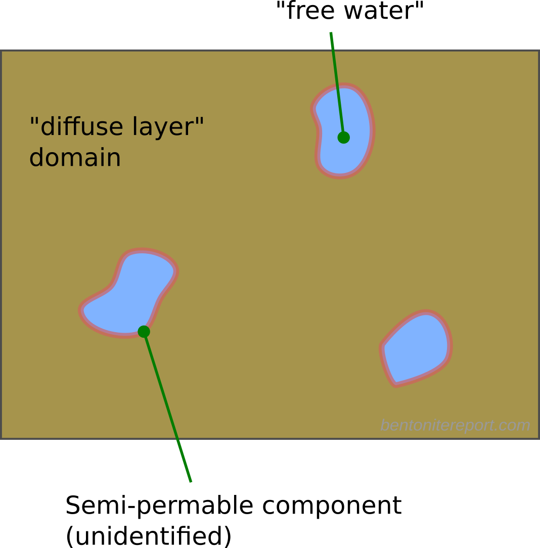
On an abstract level, we may thus illustrate a multi-porosity approach something like this (here involving two domains)

The model is represented by one continuum for the “free water”/”macroporosity” and one for the “diffuse layer”/”microporosity”,2 which are postulated to be in equilibrium within each macroscopic cell.
But such an equilibrium (Donnan equilibrium) requires a semi-permeable component. I am not aware of any suggestion for such a component in any publication on multi-porosity models. Likewise, the co-existence of diffuse layer and free water domains requires a mechanism that prevents swelling and maintains the pressure difference — also the water chemical potential should of course be the equal in the two “porosities”.3
Note that the questions of what constitutes the semi-permeable component and what prevents swelling have a clear answer in the homogeneous mixture model. This answer also corresponds to an easily identified real-world object: the metal filter (or similar component) separating the sample from the external solution. Multi-porosity models, on the other hand, attribute no particular significance to interfaces between sample and external solutions. Therefore, a candidate for the semi-permeable component has to be — but isn’t — sought elsewhere. Donnan equilibrium calculations are virtually meaningless without identifying this component.
The partitioning between diffuse layer and free water in multi-porosity models is, moreover, assumed to be controlled by water chemistry, usually by means of the Debye length. E.g. Alt-Epping et al. (2015) write
To determine the volume of the microporosity, the surface area of montmorillonite, and the Debye length, \(D_L\), which is the distance from the charged mineral surface to the point where electrical potential decays by a factor of e, needs to be known. The volume of the microporosity can then be calculated as \begin{equation*} \phi^\mathrm{EDL} = A_\mathrm{clay} D_L, \end{equation*} where \(A_\mathrm{clay}\) is the charged surface area of the clay mineral.
I cannot overstate how strange the multi-porosity description is. Leaving the abstract representation, here is an attempt to illustrate the implied clay structure, at the “macropore” scale
The view emerging from the above description is actually even more peculiar, as the “micro” and “macro” volume fractions are supposed to vary with the Debye length. A more general illustration of how the pore structure is supposed to function is shown in this animation (“I” denotes ionic strength)

What on earth could constitute such magic semi-permeable membranes?! (Note that they are also supposed to withstand the inevitable pressure difference.)
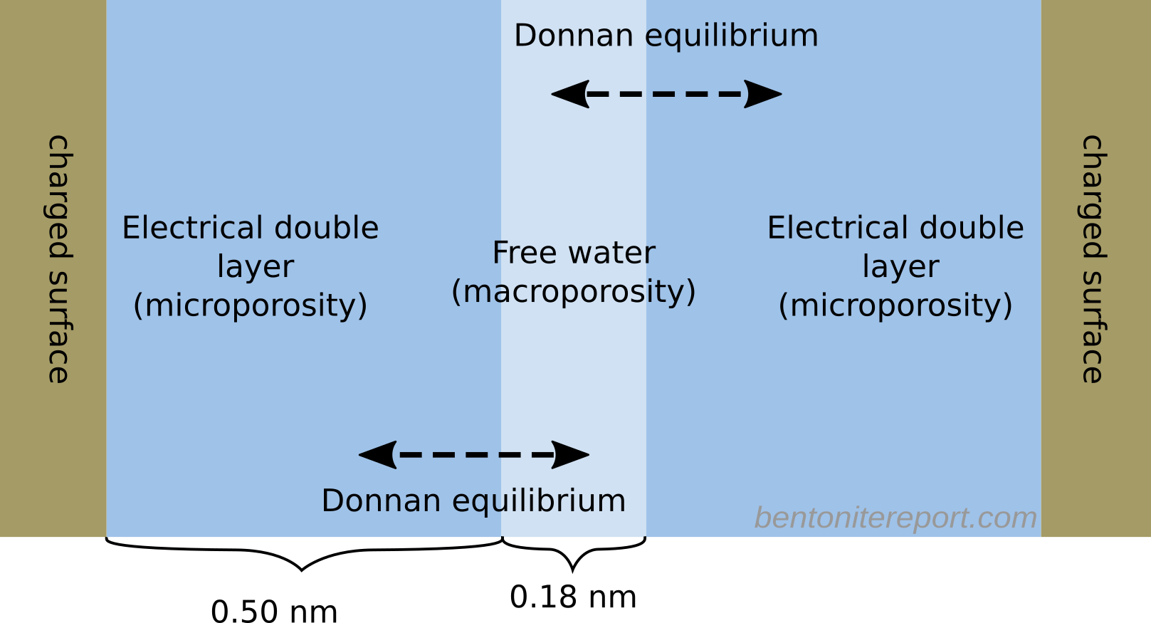
Here, the informed reader may object and point out that no researcher promoting multi-porosity has this magic pore structure in mind. Indeed, basically all multi-porosity publications instead vaguely claim that the domain separation occurs on the nanometer scale and present microscopic illustrations, like this (this is a simplified version of what is found in Alt-Epping et al. (2015))

In the remainder of this post I will discuss how the idea of a domain separation on the microscopic scale is even more preposterous than the magic membranes suggested above. We focus on three aspects:
- The implied structure of the free water domain
- The arbitrary domain division
- Donnan equilibrium on the microscopic scale is not really a valid concept
Implied structure of the free water domain
I’m astonished by how little figures of the microscopic scale are explained in many publications. For instance, the illustration above clearly suggests that “free water” is an interface region with exactly the same surface area as the “double layer”. How can that make sense? Also, if the above structure is to be taken seriously it is crucial to specify the extensions of the various water layers. It is clear that the figure shows a microscopic view, as it depicts an actual diffuse layer.4 A diffuse layer width varies, say, in the range 1 – 100 nm,5 but authors seldom reveal if we are looking at a pore 1 nm wide or several hundred nm wide. Often we are not even shown a pore — the water film just ends in a void, as in the above figure.6
The vague nature of these descriptions indicates that they are merely “decorations”, providing a microscopic flavor to what in effect still is a macroscopic model formulation. In practice, most multi-porosity formulations provide some ad hoc mean to calculate the volume of the diffuse layer domain, while the free water porosity is either obtained by subtracting the diffuse layer porosity from total porosity, or by just specifying it. Alt-Epping et al. (2015), for example, simply specifies the “macroporosity”
The total porosity amounts to 47.6 % which is divided into 40.5 % microporosity (EDL) and 7.1 % macroporosity (free water). From the microporosity and the surface area of montmorillonite (Table 7), the Debye length of the EDL calculated from Eq. 11 is 4.97e-10 m.
Clearly, nothing in this description requires or suggests that the “micro” and “macroporosities” are adjacent waterfilms on the nm-scale. On the contrary, such an interpretation becomes quite grotesque, with the “macroporosity” corresponding to half a monolayer of water molecules! An illustration of an actual pore of this kind would look something like this
This interpretation becomes even more bizarre, considering that Alt-Epping et al. (2015) assume advection to occur only in this half-a-monolayer of water, and that the diffusivity is here a factor 1000 larger than in the “microporosity”.
As another example, Appelo and Wersin (2007) model a cylindrical sample of “Opalinus clay” of height 0.5 m and radius 0.1 m, with porosity 0.16, by discretizing the sample volume in 20 sections of width 0.025 m. The void volume of each section is consequently \(V_\mathrm{void} = 0.16\cdot\pi\cdot 0.1^2\cdot 0.025\;\mathrm{m^3} = 1.257\cdot10^{-4}\;\mathrm{m^3}\). Half of this volume (“0.062831853” liter) is specified directly in the input file as the volume of the free water;7 again, nothing suggests that this water should be distributed in thin films on the nm-scale. Yet, Appelo and Wersin (2007) provide a figure, with no length scale, similar in spirit to that above, that look very similar to this

They furthermore write about this figure (“Figure 2”)
It should be noted that the model can zoom in on the nm-scale suggested by Figure 2, but also uses it as the representative form for the cm-scale or larger.
I’m not sure I can make sense of this statement, but it seems that they imply that the illustration can serve both as an actual microscopic representation of two spatially separated domains and as a representation of two abstract continua on the macroscopic scale. But this is not true!
Interpreted macroscopically, the vertical dimension is fictitious, and the two continua are in equilibrium in each paired cell. On a microscopic scale, on the other hand, equilibrium between paired cells cannot be assumed a priori, and it becomes crucial to specify both the vertical and horizontal length scales. As Appelo and Wersin (2007) formulate their model assuming equilibrium between paired cells, it is clear that the above figure must be interpreted macroscopically (the only reference to a vertical length scale is that the “free solution” is located “at infinite distance” from the surface).
We can again work out the implications of anyway interpreting the model microscopically. Each clay cell is specified to contain a surface area of \(A_\mathrm{surf}=10^5\;\mathrm{m^2}\).8 Assuming a planar geometry, the average pore width is given by (\(\phi\) denotes porosity and \(V_\mathrm{cell}\) total cell volume)
\begin{equation} d = 2\cdot \phi \cdot \frac{V_\mathrm{cell}}{A_\mathrm{surf}} = 2\cdot \frac{V_\mathrm{void}}{A_\mathrm{surf}} = 2\cdot \frac{1.26\cdot 10^{-4}\;\mathrm{m^3}}{10^{5}\;\mathrm{m^2}} = 2.51\;\mathrm{nm} \end{equation}
The double layer thickness is furthermore specified to be 0.628 nm.9 A microscopic interpretation of this particular model thus implies that the sample contains a single type of pore (2.51 nm wide) in which the free water is distributed in a thin film of width 1.25 nm — i.e. approximately four molecular layers of water!
Rather than affirming that multi-porosity model formulations are macroscopic at heart, parts of the bentonite research community have instead doubled down on the confusing idea of having free water distributed on the nm-scale. Tournassat and Steefel (2019) suggest dealing with the case of two parallel charged surfaces in terms of a “Dual Continuum” approach, providing a figure similar to this (surface charge is -0.11 C/m2 and external solution is 0.1 M of a 1:1 electrolyte)

Note that here the perpendicular length scale is specified, and that it is clear from the start that the electrostatic potential is non-zero everywhere. Yet, Tournassat and Steefel (2019) mean that it is a good idea to treat this system as if it contained a 0.7 nm wide bulk water slice at the center of the pore. They furthermore express an almost “postmodern” attitude towards modeling, writing
It should be also noted here that this model refinement does not imply necessarily that an electroneutral bulk water is present at the center of the pore in reality. This can be appreciated in Figure 6, which shows that the Poisson–Boltzmann predicts an overlap of the diffuse layers bordering the two neighboring surfaces, while the dual continuum model divides the same system into a bulk and a diffuse layer water volume in order to obtain an average concentration in the pore that is consistent with the Poisson–Boltzmann model prediction. Consequently, the pore space subdivision into free and DL water must be seen as a convenient representation that makes it possible to calculate accurately the average concentrations of ions, but it must not be taken as evidence of the effective presence of bulk water in a nanoporous medium.
I can only interpret this way of writing (“…does not imply necessarily that…”, “…must not be taken as evidence of…”) that they mean that in some cases the bulk phase should be interpreted literally, while in other cases the bulk phase should be interpreted just as some auxiliary component. It is my strong opinion that such an attitude towards modeling only contributes negatively to process understanding (we may e.g. note that later in the article, Tournassat and Steefel (2019) assume this perhaps non-existent bulk water to be solely responsible for advective flow…).
I say it again: no matter how much researchers discuss them in microscopic terms, these models are just macroscopic formulations. Using the terminology of Tournassat and Steefel (2019), they are, at the end of the day, represented as dual continua assumed to be in local equilibrium (in accordance with the first figure of this post). And while researchers put much effort in trying to give these models a microscopic appearance, I am not aware of anyone suggesting a reasonable candidate for what actually could constitute the semi-permeable component necessary for maintaining such an equilibrium.
Arbitrary division between diffuse layer and free water
Another peculiarity in the multi-porosity descriptions showing that they cannot be interpreted microscopically is the arbitrary positioning of the separation between diffuse layer and free water. We saw earlier that Alt-Epping et al. (2015) set this separation at one Debye length from the surface, where the electrostatic potential is claimed to have decayed by a factor of e. What motivates this choice?
Most publications on multi-porosity models define free water as a region where the solution is charge neutral, i.e. where the electrostatic potential is vanishingly small.10 At the point chosen by Alt-Epping et al. (2015), the potential is about 37% of its value at the surface. This cannot be considered vanishingly small under any circumstance, and the region considered as free water is consequently not charge neutral.
The diffuse layer thickness chosen by Appelo and Wersin (2007) instead corresponds to 1.27 Debye lengths. At this position the potential is about 28% of its value at the surface, which neither can be considered vanishingly small. At the mid point of the pore (1.25 nm), the potential is about 8%11 of the value at the surface (corresponding to about 2.5 Debye lengths). I find it hard to accept even this value as vanishingly small.
Note that if the boundary distance used by Appelo and Wersin (2007) (1.27 Debye lengths) was used in the benchmark of Alt-Epping et al. (2015), the diffuse layer volume becomes larger than the total pore volume! In fact, this occurs in all models of this kind for low enough ionic strength, as the Debye length diverges in this limit. Therefore, many multi-porosity model formulations include clunky “if-then-else” clauses,12 where the system is treated conceptually different depending on whether or not the (arbitrarily chosen) diffuse layer domain fills the entire pore volume.13
In the example from Tournassat and Steefel (2019) the extension of the diffuse layer is 1.6 nm, corresponding to about 1.69 Debye lengths. The potential is here about 19% of the surface value (the value in the midpoint is 12% of the surface value). Tournassat and Appelo (2011) uses yet another separation distance — two Debye lengths — based on misusing the concept of exclusion volume in the Gouy-Chapman model.
With these examples, I am not trying to say that a better criterion is needed for the partitioning between diffuse layer and bulk. Rather, these examples show that such a partitioning is quite arbitrary on a microscopic scale. Of course, choosing points where the electrostatic potential is significant makes no sense, but even for points that could be considered having zero potential, what would be the criterion? Is two Debye lengths enough? Or perhaps four? Why?
These examples also demonstrate that researchers ultimately do not have a microscopic view in mind. Rather, the “microscopic” specifications are subject to the macroscopic constraints. Alt-Epping et al. (2015), for example, specifies a priori that the system contains about 15% free water, from which it follows that the diffuse layer thickness must be set to about one Debye length (given the adopted surface area). Likewise, Appelo and Wersin (2007) assume from the start that Opalinus clay contains 50% free water, and set up their model accordingly.14 Tournassat and Steefel (2019) acknowledge their approach to only be a “convenient representation”, and don’t even relate the diffuse layer extension to a specific value of the electrostatic potential.15 Why the free water domain anyway is considered to be positioned in the center of the nanopore is a mystery to me (well, I guess because sometimes this interpretation is supposed to be taken literally…).
Note that none of the free water domains in the considered models are actually charged, even though the electrostatic potential in the microscopic interpretations is implied to be non-zero. This just confirms that such interpretations are not valid, and that the actual model handling is the equilibration of two (or more) macroscopic, abstract, continua. The diffuse layer domain is defined by following some arbitrary procedure that involves microscopic concepts. But just because the diffuse layer domain is quantified by multiplying a surface area by some multiple of the Debye length does not make it a microscopic entity.4
Donnan effect on the microscopic scale?!
Although we have already seen that we cannot interpret multi-porosity models microscopically, we have not yet considered the weirdest description adopted by basically all proponents of these models: they claim to perform Donnan equilibrium calculations between diffuse layer and free water regions on the microscopic scale!
The underlying mechanism for a Donnan effect is the establishment of charge separation, which obviously occur on the scale of the ions, i.e. on the microscopic scale. Indeed, a diffuse layer is the manifestation of this charge separation. Donnan equilibrium can consequently not be established within a diffuse layer region, and discontinuous electrostatic potentials only have meaning in a macroscopic context.
Consider e.g. the interface between bentonite and an external solution in the homogeneous mixture model. Although this model ignores the microscopic scale, it implies charge separation and a continuously varying potential on this scale, as illustrated here

The regions where the potential varies are exactly what we categorize as diffuse layers (exemplified in two ideal microscopic geometries).
The discontinuous potentials encountered in multi-porosity model descriptions (see e.g. the above “Dual Continuum” potential that varies discontinuously on the angstrom scale) can be drawn on paper, but don’t convey any physical meaning.
Here I am not saying that Donnan equilibrium calculations cannot be performed in multi-porosity models. Rather, this is yet another aspect showing that such models only have meaning macroscopically, even though they are persistently presented as if they somehow consider the microscopic scale.
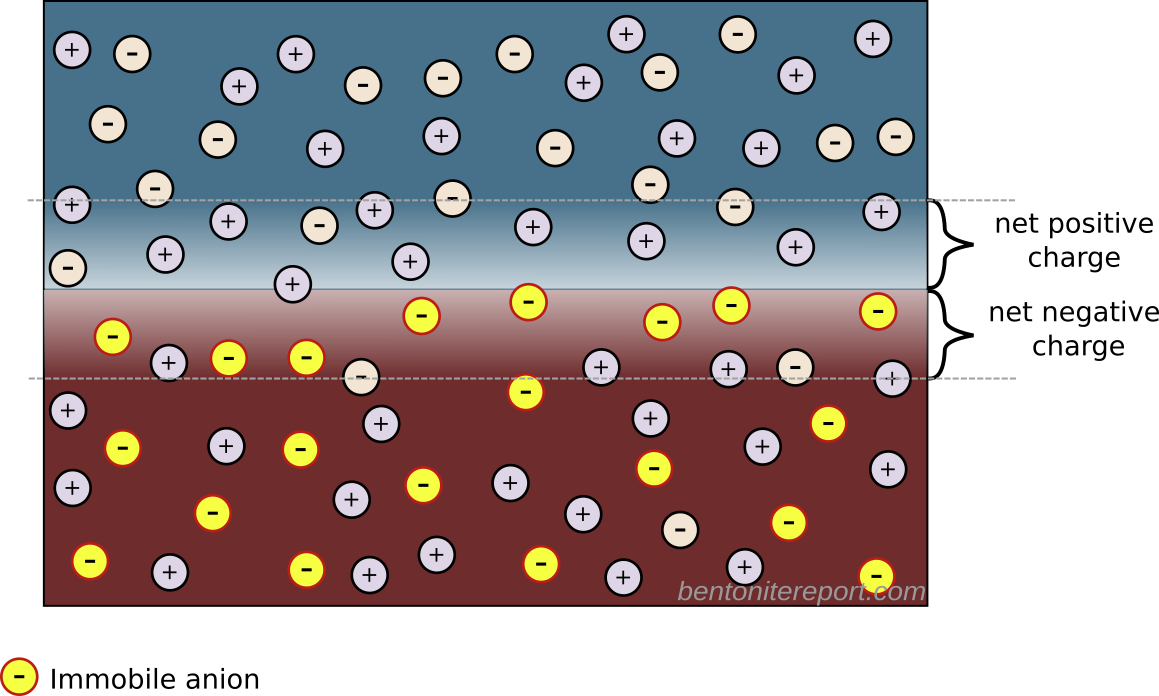
An example of this confusion of scales is found in Alt-Epping et al. (2018), who revisit the benchmark problem of Alt-Epping et al. (2015) using an alternative approach to Donnan equilibrium: rather than directly calculating the equilibrium, they model the clay charge as immobile mono-valent anions, and utilize the Nernst-Planck equations. They present “the conceptual model” in a figure very similar to this one

This illustration simultaneously conveys both a micro- and macroscopic view. For example, a mineral surface is indicated at the bottom, suggesting that we supposedly are looking at an actual interface region, in similarity with the figures we have looked at earlier. Moreover, the figure contains entities that must be interpreted as individual ions, including the immobile “clay-anions”. As in several of the previous examples, no length scale is provided (neither perpendicular to, nor along the “surface”).
On the other hand, the region is divided into cells, similar to the illustration in Appelo and Wersin (2007). These can hardly have any other meaning than to indicate the macroscopic discretization in the adopted transport code (FLOTRAN). Also, as the “Donnan porosity” region contains the “clay-anions” it can certainly not represent a diffuse layer extending from a clay surface; the only way to make sense of such an “immobile-anion” solution is that it represents a macroscopic homogenized clay domain (a homogeneous mixture!).
Furthermore, if the figure is supposed to show the microscopic scale there is no Donnan effect, because there is no charge separation! Taking the depiction of individual ions seriously, the interface region should rather look something like this in equilibrium
This illustrates the fundamental problem with a Donnan effect between microscopic compartments: the effect requires a charge separation, whose extension is the same as the size of the compartments assumed to be in equilibrium.16
Despite the confusion of the illustration in Alt-Epping et al. (2018), it is clear that a macroscopic model is adopted, as in our previous examples. In this case, the model is explicitly 2-dimensional, and the authors utilize the “trick” to make diffusion much faster in the perpendicular direction compared to the direction along the “surface”. This is achieved either by making the perpendicular diffusivity very high, or by making the perpendicular extension small. In any case, a perpendicular length scale must have been specified in the model, even if it is nowhere stated in the article. The same “trick” for emulating Donnan equilibrium is also used by Jenni et al. (2017), who write
In the present model set-up, this approach was implemented as two connected domains in the z dimension: one containing all minerals plus the free porosity (z=1) and the other containing the Donnan porosity, including the immobile anions (CEC, z=2, Fig. 2). Reproducing instantaneous equilibrium between Donnan and free porosities requires a much faster diffusion between the porosity domains than along the porosity domains.
Note that although the perpendicular dimension (\(z\)) here is referred to without unit(!), this representation only makes sense in a macroscopic context.
Jenni et al. (2017) also provide a statement that I think fairly well sums up the multi-porosity modeling endeavor:17
In a Donnan porosity concept, cation exchange can be seen as resulting from Donnan equilibrium between the Donnan porosity and the free porosity, possibly moderated by additional specific sorption. In CrunchflowMC or PhreeqC (Appelo and Wersin, 2007; Steefel, 2009; Tournassat and Appelo, 2011; Alt-Epping et al., 2014; Tournassat and Steefel, 2015), this is implemented by an explicit partitioning function that distributes aqueous species between the two pore compartments. Alternatively, this ion partitioning can be modelled implicitly by diffusion and electrochemical migration (Fick’s first law and Nernst-Planck equations) between the free porosity and the Donnan porosity, the latter containing immobile anions representing the CEC. The resulting ion compositions of the two equilibrated porosities agree with the concentrations predicted by the Donnan equilibrium, which can be shown in case studies (unpublished results, Gimmi and Alt-Epping).
Ultimately, these are models that, using one approach or the other, simply calculates Donnan equilibrium between two abstract, macroscopically defined domains (“porosities”, “continua”). Microscopic interpretations of these models lead — as we have demonstrated — to multiple absurdities and errors. I am not aware of any multi-porosity approach that has provided any kind of suggestion for what constitutes the semi-permeable component required for maintaining the equilibrium they are supposed to describe. Alternatively expressed: what, in the previous figure, prevents the “immobile anions” from occupying the entire clay volume?
The most favorable interpretation I can make of multi-porosity approaches to bentonite modeling is a dynamically varying “macroporosity”, involving magical membranes (shown above). This, in itself, answers why I cannot take multi-porosity models seriously. And then we haven’t yet mentioned the flawed treatment of diffusive flux.
Footnotes
[1] This category has many other names, e.g. “dual porosity” and “dual continuum”, models. Here, I mostly use the term “multi-porosity” to refer to any model of this kind.
[2] These compartments have many names in different publications. The “diffuse layer” domain is also called e.g. “electrical double layer (EDL)”, “diffuse double layer (DDL)”, “microporosity”, or “Donnan porosity”, and the “free water” is also called e.g. “macroporosity”, “bulk water”, “charge-free” (!), or “charge-neutral” porewater. Here I will mostly stick to using the terms “diffuse layer” and “free water”.
[3] This lack of a full description is very much related to the incomplete description of so-called “stacks” — I am not aware of any reasonable suggestion of a mechanism for keeping stacks together.
[4] Note the difference between a diffuse layer and a diffuse layer domain. The former is a structure on the nm-scale; the latter is a macroscopic, abstract model component (a continuum).
[5] The scale of an electric double layer is set by the Debye length, \(\kappa^{-1}\). From the formula for a 1:1 electrolyte, \(\kappa^{-1} = 0.3 \;\mathrm{nm}/\sqrt{I}\), the Debye length is seen to vary between 0.3 nm and 30 nm when ionic strength is varied between 1.0 M to 0.0001 M (\(I\) is the numerical value of the ionic strength expressed in molar units). Independent of the value of the factor used to multiply \(\kappa^{-1}\) in order to estimate the double layer extension, I’d say that the estimation 1 – 100 nm is quite reasonable.
[6] Here, the informed reader may perhaps point out that authors don’t really mean that the free water film has exactly the same geometry as the diffuse layer, and that figures like the one above are more abstract representations of a more complex structure. Figures of more complex pore structures are actually found in many multi-porosity papers. But if it is the case that the free water part is not supposed to be interpreted on the microscopic scale, we are basically back to a magic membrane picture of the structure! Moreover, if the free water is not supposed to be on the microscopic scale, the diffuse layer will always have a negligible volume, and these illustrations don’t provide a mean for calculating the partitioning between “micro” and “macroporosity”.
It seems to me that not specifying the extension of the free water is a way for authors to dodge the question of how it is actually distributed (and, as a consequence, to not state what constitutes the semi-permeable component).
[7] The PHREEQC input files are provided as supplementary material to Appelo and Wersin (2007). Here I consider the input corresponding to figure 3c in the article. The free water is specified with keyword “SOLUTION”.
[8] Keyword “SURFACE” in the PHREEQC input file for figure 3c in the paper.
[9] Using the identifier “-donnan” for the “SURFACE” keyword.
[10] We assume a boundary condition such that the potential is zero in the solution infinitely far away from any clay component.
[11] Assuming exponential decay, which is only strictly true for a single clay layer of low charge.
[12] For example, Tournassat and Steefel (2019) write (\(f_{DL}\) denotes the volume fraction of the diffuse layer):
In PHREEQC and CrunchClay, the volume of the diffuse layer (\(V_{DL}\) in m3), and hence the \(f_{DL}\) value, can be defined as a multiple of the Debye length in order to capture this effect of ionic strength on \(f_{DL}\): \begin{equation*} V_{DL} = \alpha_{DL}\kappa^{-1}S \tag{22} \end{equation*} \begin{equation*} f_{DL} = V_{DL}/V_{pore} \end{equation*} […] it is obvious that \(f_{DL}\) cannot exceed 1. Equation (22) must then be seen as an approximation, the validity of which may be limited to small variations of ionic strength compared to the conditions at which \(f_{DL}\) is determined experimentally. This can be appreciated by looking at the results obtained with a simple model where: \begin{equation*} \alpha_{DL} = 2\;\mathrm{if}\;4\kappa^{-1} \le V_{pore}/S\;\mathrm{and,} \end{equation*} \begin{equation*} f_{DL} = 1 \;\mathrm{otherwise.} \end{equation*}
[13] Some tools (e.g. PHREEQC) allow to put a maximum size limit on the diffuse layer domain, independent of chemical conditions. This is of course only a way for the code to “work” under all conditions.
[14] As icing on the cake, these estimations of free water in bentonite (15%) and Opalinus clay (50%) appear to be based on the incorrect assumption that “anions” only reside in such compartments. In the present context, this handling is particularly confusing, as a main point with multi-porosity models (I assume?) is to evaluate ion concentrations in other types of compartments.
[15] Yet, Tournassat and Steefel (2019) sometimes seem to favor the choice of two Debye lengths (see footnote 12), for unclear reasons.
[16] Donnan equilibrium between microscopic compartments can be studied in molecular dynamics simulations, but they require the considered system to be large enough for the electrostatic potential to reach zero. The semi-permeable component in such simulations is implemented by simply imposing constraints on the atoms making up the clay layer.
[17] I believe the referred unpublished results now are published: Gimmi and Alt-Epping (2018).