We can directly apply the homogeneous mixture model for bentonite to isolated systems — e.g. closed-cell diffusion tests — as discussed previously. For systems involving external solutions we must also handle the chemical equilibrium at solution/bentonite interfaces.

I have presented a framework for calculating the chemical equilibrium between an external solution and a bentonite component in the homogeneous mixture model here. In this post I will discuss and illustrate some aspects of that work.

Overview

We assume a homogeneous bentonite domain in contact with an external solution, with the clay particles prevented from crossing the domain interface. For real systems, this corresponds to the frequently encountered set-up with bentonite confined in a sample holder by means of e.g. a metal filter. From the assumptions of the homogeneous model — that all ions are mobile and allowed to cross the domain interface — it follows that the type of equilibrium to consider is the famous Donnan equilibrium. I have discussed the Donnan effect and its relevance for bentonite quite extensively here.

Since the adopted model assumes a homogeneous bentonite domain, the only region where Donnan equilibrium comes into play is at the interface between the bentonite and the external solution. This is quite different from how Donnan equilibrium calculations are implemented in many multi-porous models, where the equilibrium is internal to the clay — between assumed “macro” and “micro” compartments of the pore structure. The need for performing Donnan equilibrium calculations is thus minimized in the homogeneous mixture model (as mentioned, isolated systems require no such calculations). Note also that the semi-permeable mechanism in multi-porous models is required to act on the pore-scale. I have never seen any description or explanation how such a mechanism is supposed to work.¹ In the homogeneous mixture model, on the other hand, the semi-permeable interface corresponds directly to a macroscopic and experimentally well-defined component: the confining filter.

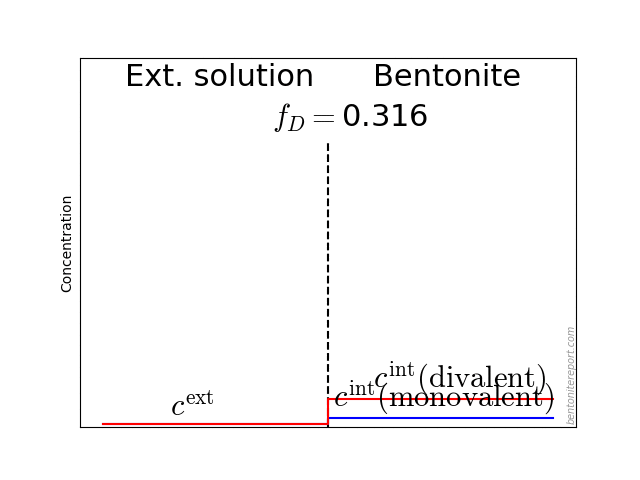
The problem to be solved can be illustrated like this

The aim is to relate the set of species concentrations in the external solution (\(\{c_i^\mathrm{ext}\}\)) to those in the clay domain (\(\{c_i^\mathrm{int}\}\)) when the system is in equilibrium. This is done by applying the standard approach to Donnan equilibrium, as found in textbooks on the subject. If there is anything “radical” about this framework, it is thus not in the way Donnan equilibrium is implemented, but rather in treating bentonite as a single phase: this approach is formally equivalent to assuming the bentonite to be an aqueous solution.

Chemical equilibrium

I prefer to formulate the Donnan equilibrium framework in a way that separates effects due to difference in the local chemical environment from effects due to differences in electrostatic potential between the two compartments. An important reason for focusing on this separation is that the local environment affects the chemistry under all circumstances, while the (relative) value of the electrostatic potential only is relevant when bentonite is contacted with an external solution. We therefore express the chemical equilibrium as

\begin{equation} \frac{c_i^\mathrm{int}}{c_i^\mathrm{ext}} = \frac{\gamma_i^\mathrm{ext}}{\gamma_i^\mathrm{int}}\cdot e^{-\frac{z_iF\psi^\star}{RT}} \tag{1} \end{equation}

This formula is achieved by setting the electro-chemical potential equal for each species in the two compartments. Here \(\gamma_i\) denotes the activity coefficient for species \(i\), and \(\psi^*\) is the electrostatic potential difference between the compartments, which we refer to as the Donnan potential.

I find it convenient to rewrite this expression using some fancy Greek letters

\begin{equation} \label{eq:chem_eq2} \Xi_i = \Gamma_i \cdot f_D^{-z_i} \tag{2} \end{equation}

Here I call \(\Xi_i = c_i^\mathrm{int}/c_i^\mathrm{ext}\) the ion equilibrium coefficient for species \(i\). This quantity expresses the essence of ion equilibrium in the homogeneous mixture model, and will appear in many places in the analysis. \(\Xi_i\) has two factors:

• \(\Gamma_i = \gamma_i^\mathrm{ext}/\gamma_i^\mathrm{int}\) expresses the chemical aspect of the equilibrium: when \(\Gamma_i\) is large (\(>1\)), the species has a chemical preference for residing in the interlayer pores, and when \(\Gamma_i\) is small (\(<1\)), the species has a preference for the external solution. In general, \(\Gamma_i\) for any specific species \(i\) is a function of all species concentrations in the system.
• \(f_D^{-z_i}\), where \(f_D = e^{\frac{F\psi^\star}{RT}}\) is a dimensionless transformation of the Donnan potential (this is basically the Nernst equation), which we here call the Donnan factor. \(f_D\) expresses the electrostatic aspect of the equilibrium, and is the same for all species. The effect on \(\Xi_i\), however, is different for species of different charge number, because of the exponent \(-z_i\) in the full expression.

I want to emphasize that eqs. 1 and 2 express the exact same thing: chemical equilibrium between the two compartments.

Illustrations

To get a feel for the quantity \(\Xi\), here is a hopefully useful animation

It may also be helpful to see the influence of \(f_D\) on the equilibrium. Since the Donnan potential is negative, \(f_D\) is less than unity and typical values in relevant bentonite systems is \(f_D \sim\) 0.01 — 0.4. Due to the exponent \(-z_i\) in eq. 2, this influence on the equilibrium looks quite different for species with different valency. For mono- and di-valent cations, the behavior looks like this (here is put \(\Gamma = 1\) for both species)

The typical behavior for cations is that the internal concentration is much larger than the corresponding external concentration (at \(f_D = 0.01\) in the above animation, the internal concentration for the di-valent cation is enhanced by a factor \(\Xi = 10 000\)!). For anions, the internal concentration is instead lower than the external concentration,² as shown here (\(\Gamma = 1\) for both species)

Equation for \(f_D\)

For a complete description, we need an equation for calculating \(f_D\). This is derived by requiring charge neutrality in the two compartments and look like

\begin{equation*} \sum_i z_i\cdot\Gamma_i \cdot c_i^\mathrm{ext} \cdot f_D^{-z_i} – c_{IL} = 0 \tag{3} \end{equation*}

where

\begin{equation*} c_{IL} = \frac{CEC}{F \cdot w} \end{equation*}

is the structural charge present in the clay (i.e. negative montmorillonite layer charge) expressed as a monovalent interlayer concentration. Here \(CEC\) is the cation exchange capacity of the clay component, \(w\) the water-to-solid mass ratio,³ and \(F\) is the Faraday constant.

The way eq. 3 is formulated implies that the external concentrations should be used as input to the calculation. This is typically the case as the external concentrations are under experimental control.

In typical geochemical systems it is required to account for aqueous species with valency at least in the range -2 — +2 (e.g. \(\mathrm{Ca}^{2+}\), \(\mathrm{Na}^{+}\), \(\mathrm{Cl}^{-}\), \(\mathrm{SO_4}^{2-}\)), which implies that the equation for calculating \(f_D\) is generally a polynomial equation of degree four or higher.

An important special case is the 1:1 system — e.g. pure Na-montmorillonite contacted with a NaCl solution — which has an equation for \(f_D\) of only degree two, and thus have a relatively simple analytical solution

\begin{equation*} f_D = \frac{c_{IL}}{2c^\mathrm{ext} \Gamma_\mathrm{Cl}} \left ( \sqrt{1+ \frac{4(c^\mathrm{ext})^2 \Gamma_\mathrm{Na}\Gamma_\mathrm{Cl}} {c_{IL}^2}} – 1 \right ) \end{equation*}

With the machinery in place for calculating the Donnan potential, here is an animation demonstrating the response in internal sodium and chloride concentrations as the external NaCl concentration is varied. In this calculation \(c_{IL} = 2\) M, and \(\Gamma_\mathrm{Na} = \Gamma_\mathrm{Cl} = 1\)

Comment on through-diffusion

To me, the last illustration makes it absolutely clear that Donnan equilibrium and the homogeneous mixture model provide the correct principal explanation for e.g. the behavior of tracer ions in through-diffusion tests. If you choose to relate the flux in through-diffusion tests to the external concentration difference — which is basically done in all published studies, via the parameter \(D_e\) — you will evaluate large “diffusivities” for cations and small “diffusivities” for anions. These “diffusivities” will, moreover, have the opposite dependence on background concentration: the cation flux diverges in the low background concentration limit,⁴ while the anion flux approaches zero.

But this behavior is seen to be caused by differently induced internal concentration gradients. If fluxes are related to these gradients — which they of course should, if you strive for an actual Fickian description — you find that the diffusivities are no different from what is evaluated in closed-cell tests. Relating the steady-state flux to the external concentration difference in the homogeneous mixture model gives (assuming zero tracer concentration on the outflow side)

\begin{equation*} j_\mathrm{ss} = -\phi\cdot D_c \cdot \nabla c^\mathrm{int} = \phi\cdot D_c \cdot\Xi\cdot \frac{c^\mathrm{source}}{L} \end{equation*}

where \(c^\mathrm{source}\) denotes the tracer concentration in the external solution on the inflow side, \(\phi\) is the porosity, \(D_c\) is the pore diffusivity in the interlayer domain, and \(L\) is the length of the bentonite sample. From the above equation can directly be identified

\begin{equation} D_e = \phi\cdot\Xi\cdot D_c \end{equation}

\(D_e\) is thus not a diffusion coefficient, but basically a measure of \(\Xi\).

Note that this explanation for the behavior of \(D_e\) does not invoke any notion of an anion accessible volume, nor any “sorption” concept for cations.⁵

Additional comments

When I first published on Donnan equilibrium in bentonite, I was a bit confused and singled out the term “Donnan equilibrium” to refer to anions only, while calling the corresponding cation equilibrium “ion-exchange equilibrium”. To refer to “both” types of equilibrium we used the term “ion equilibrium”.⁶ Of course, Donnan equilibrium applies to ions of any charge and, being better informed, I should have used a more stringent terminology. In later publications I have tried to make amends by pointing out that the process of cation exchange is part of the establishment of Donnan equilibrium.

Being new to the Donnan equilibrium world, I also invented some of my own nomenclature and symbols: e.g. I named the ratio between internal and external concentration the ion equilibrium coefficient (\(\Xi\)). Conventionally, if I now have understood correctly, this concentration ratio is referred to as the “Donnan ratio”, and is usually labeled \(r\) (although I’ve also seen \(K\)).

But the term “Donnan ratio” seems to be used slightly differently in different contexts, e.g. defined either as \(c^\mathrm{int}/c^\mathrm{ext}\) or as \(c^\mathrm{ext}/c^\mathrm{int}\), and is sometimes related more directly to the Donnan potential (if no distinction is made between activities and concentrations, we can write \(f_D^{-z_i} = c_i^\mathrm{int}/c_i^\mathrm{ext}\)). I therefore will continue to use the term “ion equilibrium coefficient” — with label \(\Xi\) — in the context of bentonite systems. This usage has also been picked up in some other clay publications. The ion equilibrium coefficient should be understood as strictly defined as \(\Xi = c^\mathrm{int}/c^\mathrm{ext}\) for any species, and never to define, or being defined by, the Donnan potential.

To emphasize the difference between effects due to the presence of a Donnan potential and effects due to different local chemical environments, I will refer to \(f_D\) as the Donnan factor. (This term does not seem to be used conventionally for any other quantity, although there are examples where it is used as a synonym for Donnan ratio.)

Finally, as in any other approach, the current framework requires a description for the activity coefficients. For activity coefficients in the external solution, there are quite a number of models already available. For the interlayer, modeling — and measuring! — activities is an open research area (at least I hope that this research area is open).

Footnotes

[1] This is just one of several major “loose ends” in most multi-porous models. I have earlier discussed the lack of treatment of swelling, and the incorrect treatment of fluxes in different domains. Update (220622): The lack of a semi-permeable component in multi-porosity models is further discussed here.

[2] This does not have to be the case in principle, if \(\Gamma\) for the anion is large, at the same time as the external concentration is not too low.

[3] Hence, it is implied that we use concentration units based on water mass (molality).

[4] What actually happens is that the transport resistance in the filters begins to dominate.

[5] Speaking of “sorption”, we have noted before that this term nowadays is used to mean any type of uptake between bulk water and some other domain (where the species may or may not be immobile). In this sense, there is “sorption” in the homogeneous mixture model (for both cations and anions), but only at interfaces to external solutions. It thus translates to a boundary condition, rather than being part of the transport dynamics within the clay (which makes life much simpler from a numeric perspective). Update (220622): The homogeneous mixture model is extended to deal with ions that truly sorbs here.

[6] It turns out Donnan himself actually used this terminology (“ionic equilibria”)