
This is the second part of the review of “Ionic Transport in Nano-Porous Clays with Consideration of Electrostatic Effects” (Tournassat and Steefel (2015) (referred to as TS15 in the following). For background and context please check the first part. That part covered the introduction and the section “Classical Fickan Diffusion Theory”. The next section is titled “Clay mineral surfaces and related properties”, and is further partitioned into two subsections. Here we exclusively deal with the first one of these subsections: “Electrostatic properties, high surface area, and anion exclusion”. It only covers three and a half journal pages, but since the article here goes completely off the rails, there is much to comment on.
“Electrostatic properties, high surface area, and anion exclusion”
As stated in the first part, I find it remarkable that the authors use general terms such as “clay minerals” when the actual subject matter is specifically systems with a significant cation exchange capacity, and montmorillonite in particular. I will continue to refer to these systems as “bentonite” in the following, disregarding the constant references to “clay minerals” in TS15.
Stacks
After having established that montmorillonite and illite have structural negative charge, it begins:
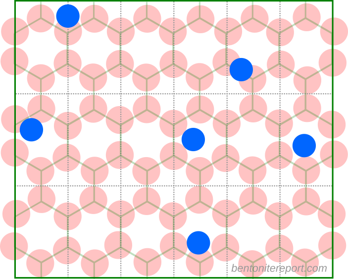
Clay mineral particles are made of layer stacks and the space between two adjacent layers is named the interlayer space (Fig. 5).
This is the first mention of clay “particles” in the article, and they are introduced as if this is a most well-established concept in bentonite science (incredibly, it is also the first occurrence of the term “interlayer”). We will refer to “clay mineral particle” constructs as “stacks” in the following. I have written a detailed post on why stacks make little sense, where I demonstrate their geometrical impossibility and show that most references given to support the concept are studies on suspensions that often imply that montmorillonite do not form stacks. Sure enough, this is also the case in TS15
The number of layers per montmorillonite particle depends on the water chemical potential and on the nature and external concentration of the layer charge compensating cation (Banin and Lahav 1968; Shainberg and Otoh 1968; Schramm and Kwak 1982a; Saiyouri et al. 2000)
Banin and Lahav (1968), Shainberg and Otoh (1968), and Schramm and Kwak (1982) all report studies on montmorillonite suspensions. The abstract of Shainberg and Otoh (1968) even states “The breakdown of the tactoids occurred when the equivalent fraction of Na increased from 0.2 to 0.5. Montmorillonite clay saturated with 50% calcium (and less) exists as single platelets.”, and the abstract of Schramm and Kwak (1982) states “Upon exchange of Ca-counterions for Li-, Na-, or K-counterions, a sharp initial decrease in tactoid size was observed over approximately the first 30% of cation exchange.”. These are just different ways of saying that sodium dominated montmorillonite is sol forming.
I want to stress the absurdity of the description given in TS15. A pure fantasy is stated about how compacted bentonite is structured. As “support” for the claim are given references to studies on “dilute suspensions”. It should be clear that the way TOT-layers interact in such suspensions essentially says nothing about how they are organized at high density. But even if we pretend that these results are applicable, the given references say that most of the relevant systems (montmorillonite with about 30% sodium or more) do not form stacks.
Disregarding the references, note also how bizarre the above statement is that the number of layers in a “particle” depends on “the water chemical potential and on the nature and external concentration of the layer charge compensating cation”: stacks are supposed to be fundamental structural units, yet the number of layers in a stack is supposed to depend on the entire water chemistry?! (It makes sense, of course, for stacks in actual suspensions.) Also, for montmorillonite an actual number of layers is nowhere stated in TS15.
TS15 further complicate things by lumping together montmorillonite and illite. In contrast to Na-montmorillonite, illite has by definition a mechanism for keeping adjacent TOT-layers together: its layer charge density is higher and compensated by potassium, which doesn’t hydrate that well, leading to collapsed interlayers. As far as I understand, one characterizing feature of illite is that the collapsed interlayers are manifested as a “10-angstrom peak” in X-ray diffraction measurements.
To treat montmorillonite and illite on equal footing (in a laid-back single sentence) again shows how nonsensical this description is. Stacking in montmorillonite suspensions occurs as a consequence of an increased ion-ion correlation effect when the fraction of e.g. calcium becomes large (> 70-80%). This process requires the ions to be diffusive and is distinctly different from the interlayer collapse in illite.
I actually have a hard time understanding what exactly is meant by the term “illite” here. In clay science it is clear that what is referred to by this name are systems that may have a quite considerable cation exchange capacity.1 Reasonably, such systems contain other types of cations besides potassium2 (as they are exchangeable), and must contain compartments where such ions can diffuse (as they are exchangeable). To increase the complexity, there are also “illite-smectite interstratified clay minerals”, which typically are in “smectite-to-illite” transitional states. For these, it seems reasonable to assume that the remaining smectite layers provide both diffusable interlayer pores and the cation exchange capacity. I don’t know if such “smectite layers” provides the cation exchange capacity in general in systems that researchers call illite. Neither do I understand how researchers can accept and use this, in my view, vague definition of “illite”. Anyway, it is the task of TS15 to sort out what they mean by the term. This is not done, and instead we get the following sentence
Illite particles typically consist of 5 to 20 stacked TOT layers (Sayed Hassan et al. 2006).
This study (Sayed Hassan et al., 2006) concerns one particular material (illite from “the Le Puy ore body”) that has been heavily processed as part of the study.3 I mean that such a specific study cannot be used as a single reference for the general nature of “illite particles”. Moreover, the stated stack size (5 — 20 layers) is nowhere stated in Sayed Hassan et al. (2006)!4
In their laid-back sentence, TS15 also implicitly define “interlayer space” as being internal to stacks. I criticized this way of redefining already established terms in the stack blog post, and TS15 serves as a good illustration of the problem: are we not supposed to be able to use the term “interlayer” without accepting the fantasy concept of stacks? To be clear, “interlayer spaces” in the context of montmorillonite simply means, and must continue to mean, spaces between adjacent TOT basal surfaces. It drives me half mad that the “stack-internal” definition is so common in contemporary bentonite scientific literature that this point seems almost impossible to communicate.
The provided illustration (“Fig 5”) explicitly shows how TS15 differ between “interlayers” that are assumed internal, and “outer basal surfaces” that are assumed external to the stack.

This illustration misrepresents the actual result of assembling a set of TOT-layers, just like any other “stack” picture found in the literature. The figure shows five identical TOT-layers that can be estimated to be smaller than 20 nm in lateral extension (while the text “conveniently” states that they should be 50 — 200 nm). Compared with “realistic” stacks, formed by randomly drawing TOT-layer sizes from an actual distribution, the depicted stack in TS15 looks like this5 (see here for details)

Besides the fact that “realistic” stack units cannot be used to form the structure of compacted bentonite, it should also be clear from this picture that “outer basal surfaces” and “interlayers” (in the sense of being internal to the stack) are not well defined. Note further that in actual compacted systems (above 1.2 g/cm3, say) such “realistic” stacks would be pushed together, something like this

In this picture, why should e.g. the interface between the green and the red stack be defined as an interface between two “outer surfaces” rather than an interlayer? Also, is this interface supposed to change nature and become an “interlayer”, as the water chemical potential or the external ion content changes? Like all other proponents of stack descriptions that I have encountered, TS15 do not in any way explain how “interlayers” and “outer surfaces” are supposed to function fundamentally differently. Similarly, they do not describe how the number of layers in a stack depends on water chemistry, nor do they provide a mechanism for why (sodium dominated) montmorillonite stacks of are supposed to keep together.
I want to emphasize that I do not favor any construction with “realistic” stacks, but only use them to illustrate the absurd consequences of taking a stack description seriously, and to demonstrate that all such descriptions in the bentonite literature are essentially pure fantasies, including the one given in TS15. I’m also quite baffled as to why TS15 (and others) provide such completely nonsensical descriptions, and how these can end up in review articles. I believe a hint is given in this formulation
[T]he number of stacked TOT layers in montmorillonite particles dictates the distribution of water in two distinct types of porosity: the interlayer porosity […] and the inter-particle porosity.
The only way I can make sense of this whole description is as an embarrassing attempt to motivate the introduction of models with several “distinct types of porosity”: the outcome is simply a macroscopic multi-porosity model (which will also be evident in later sections).
I’ve written a detailed blog post on why multi-porosity models cannot be taken seriously. There I point out that basically all authors promoting multi-porosity for some reason attempt to dress it up in terms of microscopic concepts, while the models obviously are macroscopic. Moreover, no one has ever suggested a mechanism for how equilibrium is supposed to be maintained between the different types of “porosities”.
Anion exclusion
After hallucinating about the structure of compacted bentonite, TS15 change gear and begin an “explanation” of anion exclusion. Let’s go through the description in detail.
The negative charge of the clay layers is responsible for the presence of a negative electrostatic potential field at the clay mineral basal surface–water interface.
I cannot really make sense of the term “negative electrostatic potential field”, although I think I understand what the authors are trying to say here. What is true is that the electrostatic potential near a montmorillonite basal surface is lowered compared to a point farther away. But whether or not the value of the potential is negative is irrelevant, as we are free to choose the reference level. If the zero level is chosen at a point very far from the surface, which often is done, it is true that the potential is negative at the surface. But the key principle is that the potential decreases towards the surface.6 A varying electrostatic potential signifies an electric field, which in this case is directed towards the surface (\(E = -d\phi/dx\)).
Furthermore, the electric field is not present merely because of the presence of negative charge, but because this charge is constrained to be positioned in the atomic structure of the clay. Remember that the structural clay charge is compensated by counter-ions, and that the system as a whole is charge neutral. The reason for the presence of an electric field near the surface is due to charge separation. And the reason for the potential decreasing (i.e. the electric field pointing towards the surface) is because it is the negative charge that is unable to be completely freely distributed.7
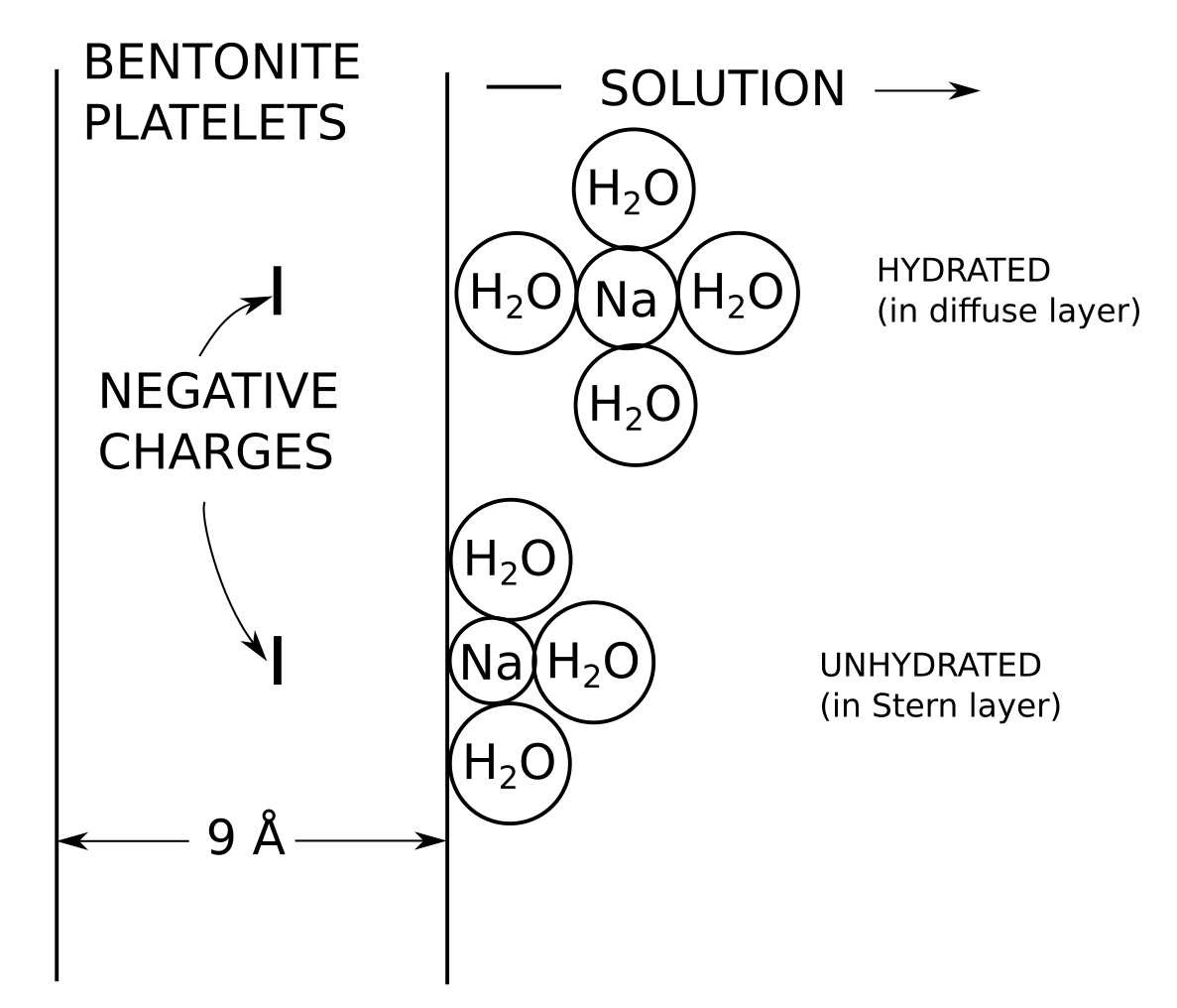
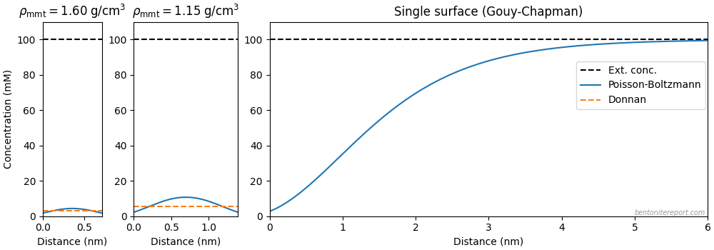
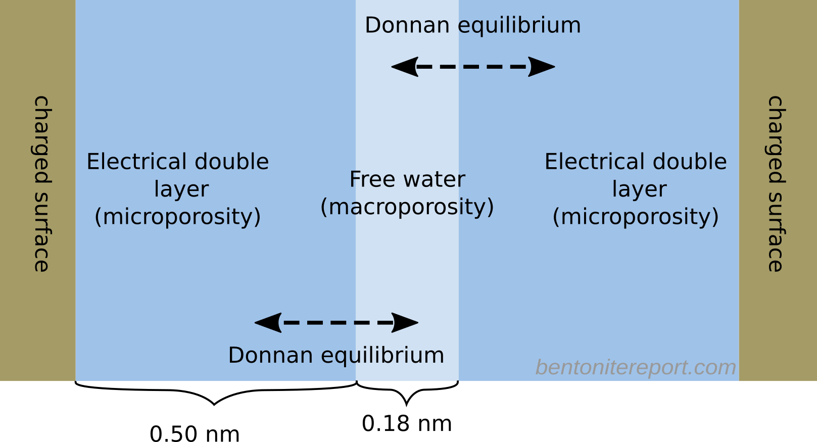
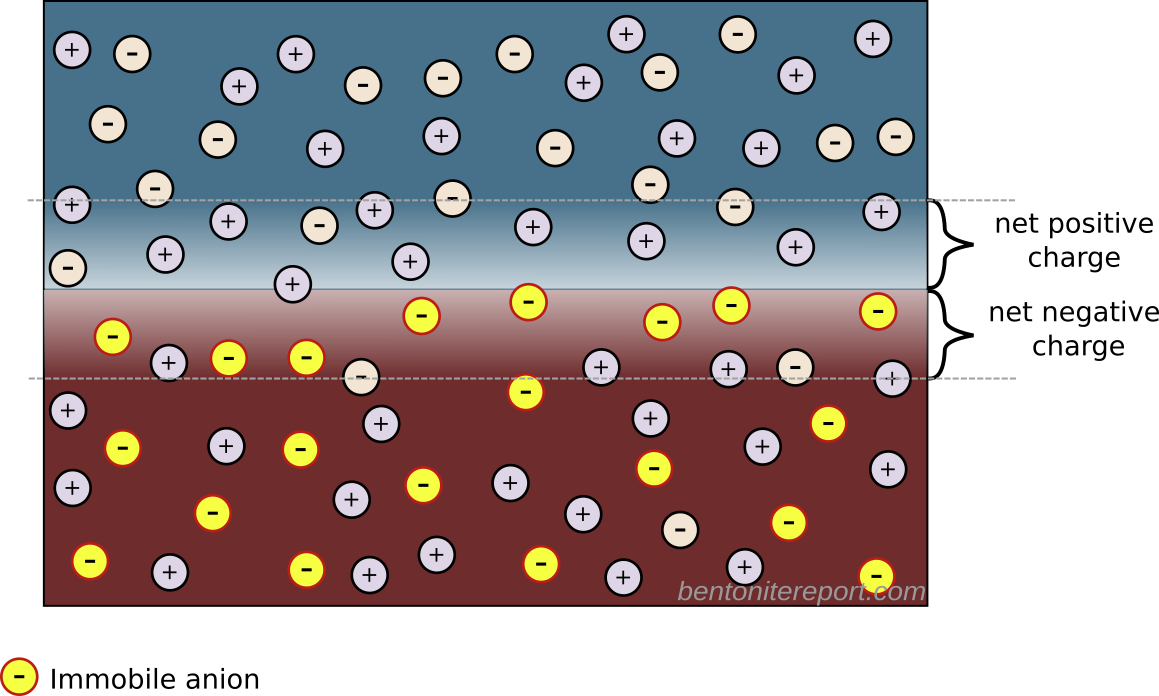
The concentrations of ions in the vicinity of basal planar surfaces of clay minerals depend on the distance from the surface considered. In a region known as the electrical double layer (EDL), concentrations of cations increase with proximity to the surface, while concentrations of anions decrease.
Having established that the electrostatic potential varies in the vicinity of the surface, it follows trivially that the ion concentrations also vary. I also find it peculiar to label the regions where the concentrations varies as the EDL. An electric double layer is a structure that includes both the surface charge and the counter-ions (hence the word “double”). What is described here should preferably be called a diffuse layer. Note, moreover, that the way an electric double layer here is introduced implies that TS15 consider a single interface, i.e. some variant of the Gouy-Chapman model (this becomes clear below). But this model is not applicable to compacted bentonite.
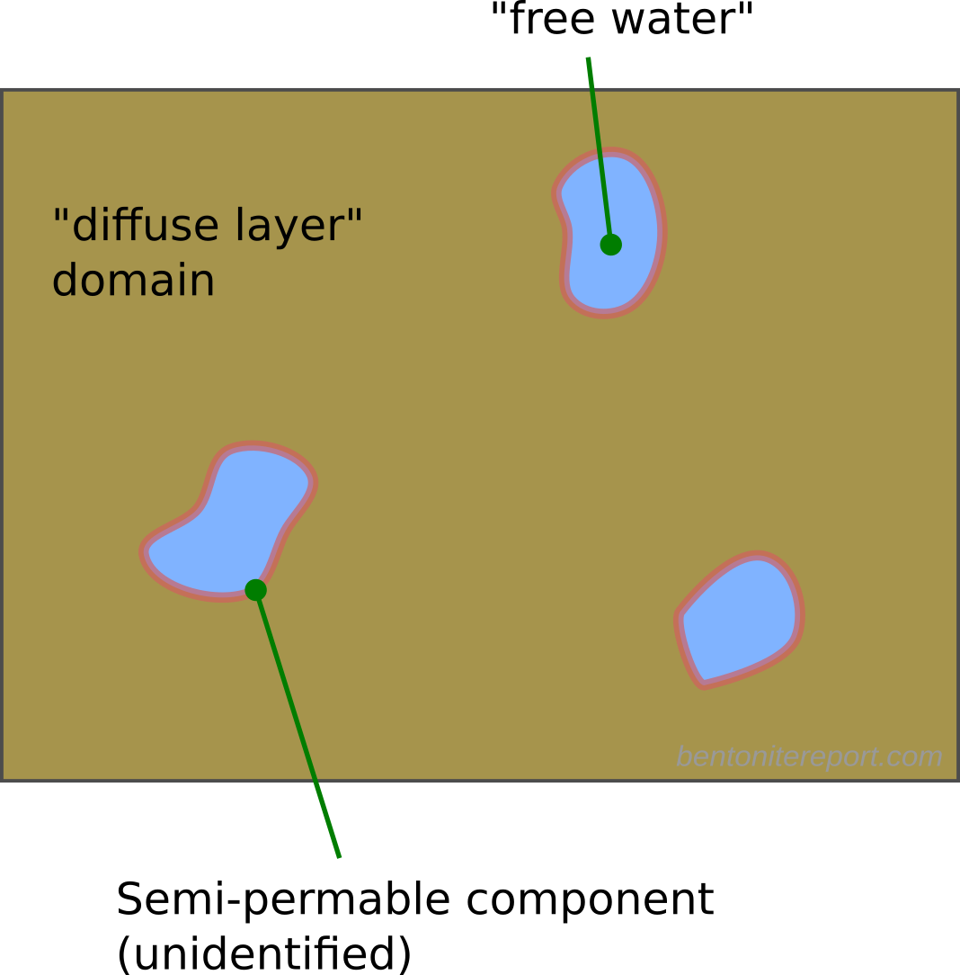
At infinite distance from the surface, the solution is neutral and is commonly described as bulk or free solution (or water).
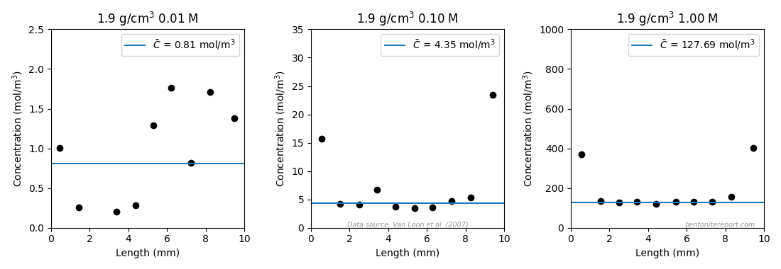
Here I think it becomes obvious that the authors try to motivate the presence of bulk water within the clay structure. As described in the blog post on “Anion accessible porosity”, it is only reasonable to assume that diffuse layers merge with a bulk solution in systems that are very sparse — i.e. in suspensions.8 This is how e.g. Schofield (1947) utilized the Gouy-Chapman model to estimate surface area. But how is the solution next to a basal surface in compacted bentonite supposed to merge with a bulk solution? Even if we use the authors’ own fantasy stack constructs, the typical structure of compacted bentonite must be envisioned something like this (I have color coded different stacks to be able to understand where they begin and end).

The regions where basal surfaces of different stacks face each other (labelled A) are way too small in order to merge with a bulk solution (and, as asked earlier, how are these regions even different from “interlayers”?). Furthermore, regions adjacent to external edge-surfaces of these imaginary stack units (B, C) are not at all considered by applying a Gouy-Chapman model. The only way to make “sense” out of the present description is to imagine larger voids in the clay structure, something like this

But even if such voids would exist (in equilibrated water-saturated bentonite under reasonable conditions, they do not) they would only constitute an exotic exception to the typical pore structure. By focusing on this type of possible “anion” exclusion, TS15 completely miss the point.
This spatial distribution of anions and cations gives rise to the anion exclusion process that is observed in diffusion experiments.
Now I’m lost. I don’t understand how ion distributions are supposed to cause a process. I think the authors here allude to Schofield’s approach to estimating surface area in montmorillonite suspensions. As discussed in detail in the blog post on anion-accessible porosity, if the suspension is so dilute that we can consider each clay layer independently, and if we equilibrate it with an external solution, we can measure its salt content, and use the Gouy-Chapman model to e.g. estimate surface area from the amount of excluded salt (as compared with the external solution).
But, as also discussed in the blog post on salt exclusion, the “Schofield type” of exclusion is not what we expect to be dominating in a dense system. Rather, in denser systems (and in Donnan systems generally — no surfaces need to be involved), salt exclusion occurs mainly because of charge separation at interfaces with the external solution. I find it revealing that TS15 so far in the article has not at all mentioned such interfaces.
Moreover, in the above sentence TS15 causally states that the anion exclusion process is “observed in diffusion experiments”, without further clarification. Given that the previous section treated diffusion, a reader would expect to have been introduced to the anion exclusion process and how it is observed in diffusion experiments. But this subsection is the first time in TS15 where the term “anion exclusion” is used! In the section on diffusion, “anion accessible porosity” was briefly mentioned, and I suppose a reader is here presumed to connect the dots. But the presence of an exclusion process certainly does not imply an “anion accessible porosity”! Furthermore, anion exclusion is not necessarily observed in diffusion experiments. A more correct statement is that we observe effects of salt exclusion in experiments where a bentonite sample is contacted with an external solution via a semi-permeable component (which typically is a filter that keeps the clay in place). The effect is most conveniently studied in equilibrium rather than diffusion tests, and salt exclusion is not present in e.g. closed-cell diffusion tests. Note that exclusion effects are always related to an external solution.
As the ionic strength increases, the EDL thickness decreases, with the result that the anion accessible porosity increases as well.
Here it is fully clear that TS15 conflate “anion accessible porosity” and “anion exclusion”. If we consider the “Schofield type” of salt exclusion, it is true that the so-called “exclusion volume” changes with the ionic strength. However, an exclusion volume is not a physical space, but an effective, equivalent quantity. It is derived from the Gouy-Chapman model, which always has anions present everywhere.
Even more importantly, the “Schofield type” of exclusion is not really of interest in dense systems (nor is the Gouy-Chapman model valid in such systems). As discussed above, one must instead consider salt exclusion stemming from charge separation at interfaces with the external solution. For this case it does not even make sense to define an exclusion volume.
I can only interpret this entire paragraph as another fruitless attempt to motivate a multi-porous modeling approach. In this subsection we have so far been told that “two distinct types of porosity” can be defined (they cannot), and we have vaguely been hinted that “bulk or free solution” also is relevant for modelling compacted bentonite. And with the last quoted sentence it is relatively clear that TS15 try to establish that the relative sizes of various “porosities” are controlled by a simple parameter (ionic strength).
The final paragraph of this subsection contain several statements that makes my jaw drop.
An equivalent anion accessible porosity can be estimated from the integration of the anion concentration profile (Fig. 6) from the surface to the bulk water (Sposito 2004)
Here the authors suddenly use the phrase “equivalent”! They are thus obviously aware of that “anion accessible porosity” is a spurious concept?! ?!?! I really don’t know what to say. Their own graph (“Fig. 6”) even show that the Gouy-Chapman model has anions (salt) everywhere! Note that this statement also implies that “the bulk water” is assumed to exist within the clay.
In compacted clay material, the pore sizes may be small as compared to the EDL size. In that case, it is necessary to take into account the EDLs overlap between two neighbouring surfaces.
I think this is a very revealing passage. The conditions of compacted bentonite are treated as an exception: pore sizes “may” be smaller than the EDL, and “in that case” it is necessary to account for overlapping diffuse layers. But for compacted bentonite, this is the only relevant situation to consider! Without “overlapping” diffuse layers there is no swelling and no sealing properties. An entire page has been devoted to discussing a model only relevant for suspensions (Gouy-Chapman), while “compacted clay material” here is commented in two sentences…
Clay mineral particles are, however, often segregated into aggregates delimiting inter-aggregate spaces whose size is usually larger than inter-particle spaces inside the aggregates.
All of a sudden — in the middle of a paragraph — we are introduced to a new structural component! “Aggregates” have not been mentioned earlier in the article and is here introduced without any references. It is my strong opinion that this way of writing is not appropriate for a scientific publication, especially not for a review article. I’m not sure what type of system the authors have in mind here, but “aggregates” are typically not present in actual water saturated bentonite. I have commented more on this in the blog post on stacks.
Conclusion
At the end of the previous section (on diffusion), we were promised that this section should qualitatively link “fundamental properties of the clay minerals” to the diffusional behavior of compacted bentonite. Instead, we are given a fictional description of the structure (conflated with structures of other “clay minerals”), along with a confused explanation of anion exclusion that is irrelevant for such systems. Not a single word is said about the equilibrium that must be considered, namely that at interfaces between bentonite and external solutions. Rather, the idea of “overlapping” diffuse layers — which is the ultimate cause for bentonite swelling — is treated as an exception and only commented on in passing (and nothing is said about how to handle such systems). Although nothing is fully spelled out, I can only interpret this entire part as a (failed) attempt to motivate a multi-porous approach to modeling bentonite. And multi-porosity models cannot be taken seriously.
I admit that scrutinizing studies and pointing out flaws can be fun. However, considering that the descriptions in TS15 are the rule rather than the exception in contemporary bentonite research, I mostly feel weary and resigned. I don’t mean that every clay researcher must agree with me that a homogeneous model is the only reasonable starting point for describing compacted bentonite, and I could only wish that this blog was more influential. But I feel almost dizzy thinking about how this research sector is so hermetically sealed that one can spend entire careers in it without ever having to worry about understanding the nature of swelling and swelling pressure.
Footnotes
[1] The Wikipedia article on illite, for example, states that the cation exchange capacity is typically 0.2 — 0.3 eq/kg. Is a significant cation exchange capacity required for classifying something as illite?
[2] E.g. (Poinssot et al., 1999), that TS15 reference as a source on illite, work with sodium exchanged “illite du Puy”, i.e. “Na-illite”.
[3] The material was dispersed by diluting it in alkaline solution and sonicating it. It was thereafter dropped as a suspension on a glass slide and dried.
[4] We may note that the number 5 — 20 TOT-layers in a stack actually showed up when we investigated how this concept is (mis)used in descriptions of bentonite. There it turned out to be a complete misunderstanding of the behavior of suspensions of Ca-montmorillonite.
[5] I am not capable to produce anything reasonable in 3D, but I think a 2D representation still conveys the message.
[6] Perhaps this criticism can be regarded as nitpicking. I have a nagging feeling, though, that electrostatics is quite poorly understood in certain parts of the bentonite research field. Take the phrase “negative electrostatic potential field”, for example. Although it can be understood at face value (a scalar field with negative values), it also appear to mix together stuff related to charges (“negative”), electric fields (“field”), and potentials. It certainly is important to separate these concepts. There are many examples in the clay literature when this is not done. E.g. Madsen and Müller-Vonmoos (1989) mean that two “potential fields” can repel each other (and also misunderstand swelling)
A high negative potential exists directly at the surface of the clay layer. […] When two such negative potential fields overlap, they repel each other, and cause the observed swelling in clay.
Horseman et al. (1996) claim that a potential repels charges:
[…] the net negative electrical potential between closely spaced clay particles repel anions attempting to migrate through the narrow aqueous films of a compact clay […]
And Shackleford and Moore (2013) mean that “overlapping” potentials repel charges
In this case, when the clay is compressed […] to the extent that the electrostatic (diffuse double) layers surrounding the particles overlap, the overlapping negative potentials repel invading anions such that the pore becomes excluded to the anion.
[7] An isolated layer of negative charge of course also has an electric field directed towards it, but this is not the relevant system to consider here. (Such a system will actually have an electric field strength that is independent of the distance to the surface, as long as the layer can be regarded as infinitely extended.)
[8] See also this comment, and this quotation.


