Here’s an opinion: The compacted bentonite research field is currently in a terrible state.
After a period away, I’ve recently begun catching up on newly published research in this field. With a fresh perspective, yet still influenced by writing over 30 long-reads over the past years, I can’t help but wonder: what is the problem? Why are a majority of researchers stuck with a view of bentonite1 that essentially makes no sense? And why has this view been the mainstream for decades now?
I get how this might come across: a solitary man ranting on a blog, criticizing an entire research field in less-than-perfect English. I probably smell bad and have some wild ideas about why General Relativity is wrong as well. But what I’m aiming for with this blog is simply a platform to present an alternative to the mainstream, primarily because it annoys me as a science-minded person how absurd this view is.2 I understand that I will likely struggle to convince anyone who is already invested in this view, but I’m trying to put myself in the shoes of e.g. someone entering this field for the first time.
For these reasons, I will try something a little new here: reviewing already published papers. I have touched on this in various forms before, but then usually with a broader topic in mind. Now I intend to critically assess specific publications from the outset. As a first publication to review in this way, I have chosen “Ionic Transport in Nano-Porous Clays with Consideration of Electrostatic Effects” (Tournassat and Steefel, 2015), for the following reasons
- It is published in “Reviews in Mineralogy & Geochemistry”, which claims that “The content of each volume consists of fully developed text which can be used for self-study, research, or as a text-book for graduate-level courses.” If anyone aims to learn about ion transport in bentonite from this publication, I would certainly recommend to also consider this review.
- It is a quite comprehensive source for many of the claims of the contemporary mainstream view that I have described in earlier blog posts. I guess it makes sense for a publication in “Reviews in Mineralogy & Geochemistry” to reflect the typical view of a research field.
- It considers the seeming uphill diffusion effect that I recently commented on. The effect is as misunderstood in this publication as it is in Tertre et al. (2024).
- It is published as open access. The article is thus accessible to anyone who wants to check the details.
I will use the abbreviation TS15 in following to refer to this publication.
Overview
The article covers 38 journal pages (+ references) and includes quite a lot of topics. At the highest level of headings, the outline look like this
- Introduction (p. 1 — 2)
- Classical Fickian Diffusion Theory (p. 2 — 9)
- Clay mineral surfaces and related properties (p. 9 — 17)
- Constitutive equations for diffusion in bulk, diffuse layer, and interlayer water (p. 17 — 23)
- Relative contributions of concentration, activity coefficient and diffusion potential gradients to total flux (p. 24 — 28)
- From diffusive flux to diffusive transport equations (p. 28 — 33)
- Applications (p. 33 — 37)
- Summary and Perspectives (p. 37 — 38)
Given the quite large scope of TS15, I will present this review in parts, with this first part focusing on the introduction and the section titled “Classical Fickian Diffusion Theory”.
“Introduction”
I find it remarkable that the authors use terms like “clays” and “clay minerals” when speaking of properties such as “low permeability”, “high adsorption capacity” and “swelling behavior”, and of applications such as nuclear waste storage. I mean that using such general terms here is too broad, as the article focuses solely on systems with swelling/sealing ability. Such an ability is generally connected to a significant cation exchange capacity. Here, I will refer to such systems as “bentonite”, although I am aware that I use the term quite sloppily. But I think this is better than to refer to the components as general “clay minerals” — I don’t think anyone consider it a good idea to e.g. use talc or kaolinite as buffer materials in nuclear waste repositories. Moreover, most of the examples considered in the article are systems that can be described as bentonite. Given the title of the article I also expect a definition of “nano-porous clays”. It is not given here, and the term is actually not used at all in the entire text! (Except one time at the very end.)
After providing a brief overview of the application of (sealing) clay materials, the introduction takes, in my opinion, a rather drastic turn (it happens without even changing paragraphs!).
Clay transport properties are however not simple to model, as they deviate in many cases from predictions made with models developed previously for “conventional” porous media such as permeable aquifers (e.g., sandstone). […] In this respect, a significant advantage of modern reactive transport models is their ability to handle complex geometries and chemistry, heterogeneities and transient conditions (Steefel et al. 2014). Indeed, numerical calculations have become one of the principal means by which the gaps between current process knowledge and defensible predictions in the environmental sciences can be bridged (Miller et al. 2010).
I think the first sentence is too subjective and general. Given the above discussion, here the term “clay transport properties” can cover a million things, if read at face value. Are all of them difficult to model? Also, something does not have to be more difficult just because it deviates from the “convention”. I would argue that several aspects of bentonite actually make it easier to model than, say, sandstone. Advective processes, for example, can often be neglected in compacted bentonite.
I find the statement regarding the advantage of reactive transport models highly problematic. Not only does it read more like an advertisement for the authors’ own tools than “fully developed text for self-study”, but the authors also seem ignorant of issues like the dangers of overparameterization (a theme that will recur).
“Classical Fickian Diffusion Theory”
As the title of the next section is “Classical Fickian Diffusion Theory,” a reader expects a discussion focused solely on diffusive process, especially when the immediate subtitle reads “Diffusion Basics.” I therefore find it peculiar that this section actually presents the traditional diffusion-sorption model, which describes a combination of diffusion and sorption processes. The model is summarized in eq. 10 in TS15
\begin{equation} \frac{\partial c}{\partial t} = \frac{D_e} {\phi + \rho_dK_D} \nabla ^ 2 c \end{equation}
where \(c\) is the “pore water” concentration of the considered species, \(D_e\) its “effective diffusivity”, \(K_D\) the sorption partition coefficient, \(\rho_d\) dry density, and \(\phi\) porosity.3 For later considerations we also note that TS15 define the denominator on the right hand side as the “rock capacity factor”, \(\alpha = \phi + \rho_dK_D\).
I find it particularly odd that two of the fundamental assumptions of this specific model are essentially left uncommented, namely that sorbed ions are immobilized and that the pores contain bulk water. Instead, the authors appear to question the assumption of Fickian diffusion in the context of clay systems, i.e. that diffusive fluxes are assumed proportional to corresponding aqueous concentration gradients.
This section aims, as far as I can see, to point out shortcomings in the description of diffusion in bentonite, and to motivate further model development. But it should be clear from the outset that using the traditional diffusion-sorption model as the basis for such an endeavor is doomed to fail. The reason for this failure is not due to assuming Fickian diffusion, but due to the other two model assumptions; it has long been demonstrated that exchangeable ions are mobile, and the notion that compacted bentonite contains mainly bulk water is absurd.
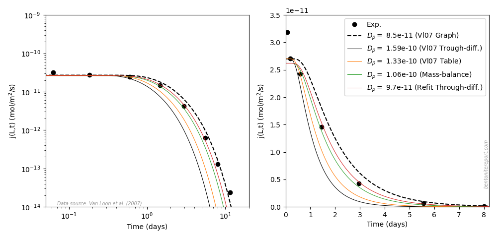
After the traditional diffusion-sorption model has been presented, it is evaluated by investigating how it can be fitted to tracer through-diffusion data (this is restatement of original work of Tachi and Yotsjui (2014)). Not surprisingly, it turns out that fitted diffusion coefficients may be unrealistically large. This is of course a direct consequence of the incorrect assumption of immobility in the traditional diffusion-sorption model. TS15 also appear to dismiss the model, saying
This result […] is not physically correct and points out the inconsistency of the classic Fickian diffusion theory for modeling diffusion processes in clay media.
I am bothered, though, that they keep using the phrase “classic Fickian diffusion theory”, which inevitably focuses on the Fickian aspect rather than on the obviously incorrect assumptions of the chosen model. Also, rather than simply concluding that the model is incorrect, TS15 continues4
[T]he large changes of \(\mathrm{Cs}^+\) diffusion parameters as a function of chemical conditions (\(D_{e,\mathrm{Cs}^+}\) decreases when the ionic strength increases […]) highlight the need to couple the chemical reactivity of clay materials to their transport properties in order to build reliable and predictive diffusion models.
There is no rationale for such a conclusion. I don’t even completely understand what “couple the chemical reactivity of clay materials to their transport properties” mean. Isn’t that what the traditional diffusion-sorption model attempts? What unrealistic \(D_e\) values actually highlights is simply that one should not use a model that assumes immobilization of “sorbed” ions.
To make things worse, TS15 describe the seeming uphill diffusion test and comment
However, the experimental observations were completely different: \(^{22}\mathrm{Na}^+\) accumulated in the high NaCl concentration reservoir as it was depleted in the low NaCl concentration reservoir, evidencing non-Fickian diffusion processes.
This is plain wrong. As explained in detail in an earlier post, the diffusion process in the “uphill” test is certainly Fickian. What the test demonstrates is, again, that “sorbed” ions are not immobile.
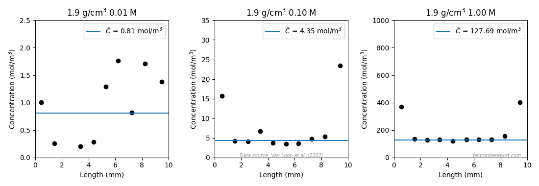
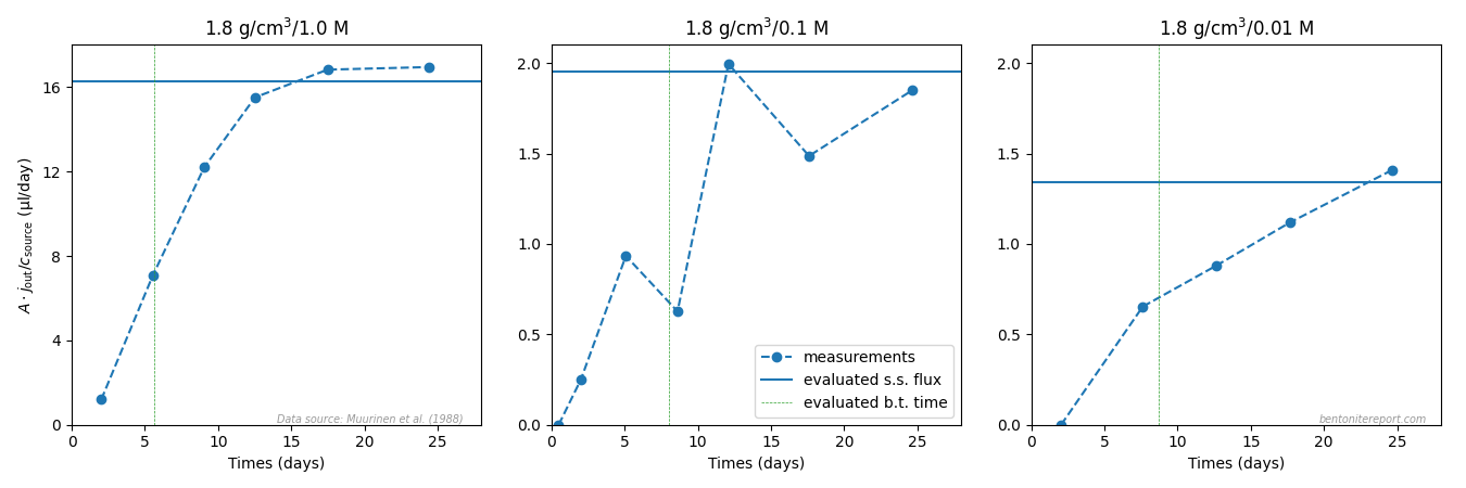
TS15 also comment on the results of fitting the model to anion tracer through-diffusion data. Here, as is well known, the fitted “rock capacity factor” \(\alpha = \phi + \rho_dK_D\) becomes significantly lower than the porosity \(\phi\). From the perspective of the traditional diffusion-sorption model, this is completely infeasible, as it implies a negative \(K_D\). But rather than simply dismissing the model, TS15 state
The lower \(\alpha\) values for anions than for water indicate that anions do not have access to all of the porosity.
Also this is incorrect. The porosity5 is an input parameter rather than a fitting parameter in the traditional diffusion-sorption model. When claiming that a small value of \(\alpha\) indicates a decreased porosity, TS15 reinterpret the parameter, on the fly, in terms of a completely different model: the effective porosity model. This model has not been mentioned at all earlier in the article.6
As has been discussed earlier on the blog, the effective porosity model can be fitted to anion tracer through-diffusion data, but now we need to keep track of two different models in the evaluation (something that TS15 do not). Moreover, these two models (the traditional diffusion-sorption and the effective porosity models) are incompatible. But TS15 continue by saying
This result is a first direct evidence of the limitation of the classic Fickian diffusion theory when applied to clay porous media: it is not possible to model the diffusion of water and anions with the same single porosity model. The observation of a lower \(\alpha\) value for anions than for water led to the development of the important concept of anion accessible porosity […]
This is a terrible passage. To begin with, the “Fickian” aspect is also here implied as the problem. But the reason for why the traditional diffusion-sorption model cannot be fitted to anion tracer through-diffusion data is of course because this model assumes the entire pore space to be filled with bulk water. Further, it’s hardly comprehensible what the authors mean by “it is not possible to model the diffusion of water and anions with the same single porosity model”. I think they simply mean that for water you must choose \(\alpha = \phi\), while for anion through-diffusion you instead must “choose” \(\alpha < \phi\). But the result \(\alpha < \phi\) should only lead to the conclusion that the traditional diffusion-sorption model cannot in any reasonable sense be fitted. A favorable reading of this passage is to assume that the authors actually mean that the effective porosity model can only be fitted to anion and water tracer through-diffusion data by using different values of the (effective) porosity, and that any “rock capacity factor” should not appear in this discussion.
Finally, the last sentence gives me headache. Rather than being an “important concept”, I mean that the idea of an “anion accessible porosity” has caused tremendous damage to the development of the bentonite research field for several decades now. We have earlier discussed on the blog that the whole idea of “anion accessible porosity” is based on misunderstandings. We have also demonstrated that the effective porosity model is not valid, even though it can be fitted to anion tracer through-diffusion data. A simple way to see this is to consider closed-cell diffusion data rather than through-diffusion data. Closed-cell tests are simpler than through-diffusion tests, as they don’t involve interfaces between clay and external solutions. We can e.g. take a look at the vast amount of diffusion coefficients for chloride in montmorillonite, presented in Kozaki et al. (1998).
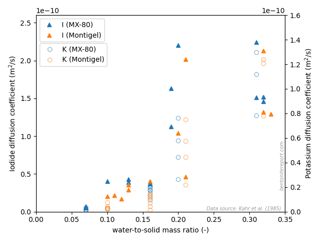
There are in total 55(!) values, corresponding to 55(!) separate tests. These have been systematically varied with respect to density and temperature, but all of them were performed on montmorillonite equilibrated with distilled water. From the perspective of the effective porosity model, the effective porosity in such a system should be minute, perhaps even strictly zero; effective porosities evaluated from chloride through-diffusion tests are well below 1% even at a background concentration as large as 10 mM. Thus, if the idea of “anion accessible porosity” was reasonable, we’d expect extremely low values of the chloride diffusion coefficient in the above plot.7 We’d perhaps also expect a threshold behavior, where chloride diffusivity basically vanishes above a certain density. But this is not at all the behavior: chloride is seen to diffuse just fine in all 55(!) tests, with temperature- and density dependencies that seems reasonable for a homogeneous system. Moreover, chloride behaves very similarly to e.g. sodium, as seen here
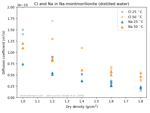
Here the sodium data is from Kozaki et al. (1998),8 and it has also been measured in montmorillonite equilibrated with distilled water.
The effective porosity model and the notion of “anion accessible porosity” can consequently be dismissed directly, by comparing with simpler tests than what is done in TS15. The reason that the effective porosity model can be fitted to anion through-diffusion data must be attributed to a misinterpretation of such tests, as they involve also interfaces to external solutions. At least to me it is completely clear that what many researchers interpret as an effective porosity is actually effects of interface equilibrium.
If TS15 were serious about evaluating bentonite diffusion processes in this section I think they should have done the following:
- Discuss the assumptions of ion immobility of sorbed ions and bulk pore water when presenting the traditional diffusion-sorption model. Moreover, they should not call this “Classical Fickian Diffusion Theory”.
- Also present and discuss the effective porosity model, as they obviously use it in their evaluations. They actually even seem to promote it! And it is as “Fickian” as the traditional diffusion-sorption model.
- Evaluate the models using closed-cell data to avoid misinterpretations arising from complications at bentonite/external solution interfaces.
- Conclude that the traditional diffusion-sorption model is not valid for bentonite, and that this is because of the assumptions of immobility of sorbed ions and bulk pore water.
- Conclude that the effective porosity model is not valid for bentonite, and that the notion of “anion accessible porosity” is flawed.
Instead, we get a quite confused and incomplete description, mixed with entirely inaccurate statements. In the end, it is difficult to understand what the takeaway message of this section really is. A reader is left with an impression that there is some problem with the “Fickian” aspect of diffusion, but nothing is spelled out. We have also been hinted that “anion accessible porosity” is important, without really having been introduced to the concept/model.
The section ends with the following passage
The limitations of the classic Fickian diffusion theory must find their origin in the fundamental properties of the clay minerals. In the next section, these fundamental properties are linked qualitatively to some of the observations described above.
If “classic Fickian diffusion theory” here is interpreted as “the traditional diffusion-sorption model” (which is literally what has been presented), the first sentence is both incorrect and trivial at the same time. The traditional diffusion-sorption model does not have “limitations” — it is fundamentally incorrect as a model for bentonite. The reason for this is that exchangeable ions are not immobile and that bentonite does not contain significant amounts of bulk water. Both of these reasons can be linked to “fundamental properties” of some specific clay minerals.
But it is clear that TS15 also have vaguely promoted the concept of “anion accessible porosity” and the effective porosity model. Are these not included in “the classic Fickian diffusion theory”? If not, why then is a model that assumes sorption and immobilization?
How can it not be immediately obvious to everyone that the diffusion process is much simpler than the contemporary descriptions?
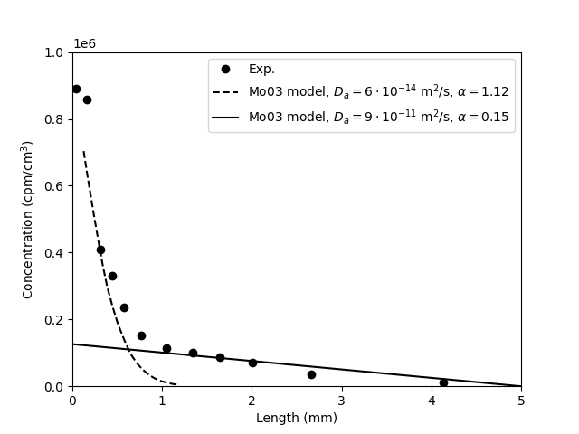
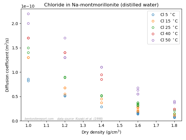
As we have brought up the data from Kozaki et al. (1998), I would like to end this blog post by further considering actual profiles of chloride and sodium diffusing in montmorillonite.
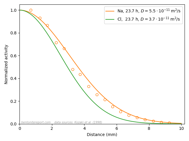
This figure shows the corresponding normalized concentration profiles after 23.7 hours in closed-cell tests performed at \(50\;^\circ\mathrm{C}\) in Na-montmorillonite at dry density \(1.8 \;\mathrm{g/cm^3}\) that has been equilibrated with distilled water. In the case of sodium, both the profile evaluated from Fick’s second law (orange line) and measured values (circles) are plotted. In the case of chloride, no measured values are available, but the value of the diffusion coefficient is the result of fitting Fick’s second law (green line) to such data.
From the perspective of the traditional diffusion-sorption model, the sodium profile is supposed to represent the combined result of ions diffusing in bulk water, at a rate many orders of magnitude larger than in pure water, while being strongly retarded due to sorption onto “the solid” (where the ions are immobile). This is clearly nonsense, and something that I think TS15 actually tries to communicate.
From the perspective of the effective porosity model, on the other hand, the chloride profile is supposed to be the result of the ion diffusing in an essentially infinitesimal fraction of the pore volume, which magically is perfectly interconnected in all samples on which such tests are conducted. This is of course just as nonsensical as the above interpretation of the sodium profile, but in this case TS15 appear to promote the model (the “important concept of anion accessible porosity”).
Note that these two simple ions, at the end of the day, diffuse very similarly (please stop reading for a moment and contemplate the above plot). If sodium and chloride actually migrate in completely different domains and are subject to completely different physico-chemical processes, this “coincident” would be more than a little weird. Especially given that the two ions show similar diffusive behavior across a wide range of densities. To me, this simple observation makes is evident that ion diffusion in bentonite at the basic level is much simpler than what is suggested by the contemporary mainstream view. I mean that it is completely obvious that all ions in bentonite diffuse in the same type of quite homogeneous domain. And since it cannot be argued that the pore volume is dominated by anything other than interlayers at 1.8 g/cm³, this homogeneous domain is the interlayer domain at any relevant density. The evidence has been available for at least 25 years (in fact much longer than that). How can this be difficult to grasp?
Update (250213): Part II of this review is found here.
Footnotes
[1] By “bentonite” I here mean any type of smectite-rich system with a significant cation exchange capacity.
[2] The irony is that the “alternative” in a broader perspective is more mainstream than the “mainstream” view. I basically propose to obey the laws of thermodynamics.
[3] I have simplified the notation here somewhat compared with how it is written in TS15. As many others, TS15 call this equation “Fick’s second law” (via their eq. 4), which is not correct. Fick’s laws refer strictly to pure diffusion processes. However, the equation has the same form as Fick’s second law, if \(D_e/(\phi + \rho_d K_D)\) is treated as a single constant (often referred to as the apparent diffusivity).
[4] This behavior is of course not unique for cesium; I don’t know why TS15 focus so hard on that ion here.
[5] “Porosity” is a volume ratio. I’m not a fan of that the word has also begun to mean “pore space” in the bentonite scientific literature.
[6] In fact, \(\alpha\) has earlier in the article been unambiguously related to sorption:
If the species \(i\) is also adsorbed on or incorporated into the solid phase, then it is possible to define a rock capacity factor \(\alpha_i\) that relates the concentration in the porous media to the concentration in solution
[7] That the diffusivity is much too large for an effective porosity interpretation to make sense can also be seen from invoking Archie’s law, which is quite popular in bentonite scientific papers.
\begin{equation} D_e = \epsilon_\mathrm{eff}^n D_0\end{equation}
Here \(D_0\) is the diffusivity in pure bulk water, which is about \(2\cdot 10^{-9} \;\mathrm{m^2/s}\) for chloride. Using the popular choice \(n \approx 2\) and choosing e.g. \(\epsilon_\mathrm{eff} = 0.001\) (most probably an overestimation when using distilled water), we get
\begin{equation} D_0 = (5.1\cdot 10^{-11} \;\mathrm{m^2/s})/0.001 = 5.1\cdot 10^{-8} \;\mathrm{m^2/s}\end{equation}
This is more than twenty times the actual value for \(D_0\). (\(D_e = 5.1\cdot 10^{-14} \;\mathrm{m^2/s}\) is evaluated from Kozaki’s data at \(1.4 \;\mathrm{g/cm^3}\) and \(25\;^\circ\mathrm{C}\))
[8] Note! This publication is different from the chloride study.