
In the ongoing assessment of chloride equilibrium concentrations in bentonite, we here take a closer look at the study by Van Loon et al. (2007), in the following referred to as Vl07. We thus assess the 54 points indicated here (click on figures to enlarge)

Vl07 is centered around a set of through-diffusion tests in “KWK” bentonite samples of nominal dry densities 1.3 g/cm3, 1.6 g/cm3, and 1.9 g/cm3. For each density, chloride tracer diffusion tests were conducted with NaCl background concentrations 0.01 M, 0.05 M, 0.1 M, 0.4 M, and 1.0 M. In total, 15 samples were tested. The samples are cylindrical with diameter 2.54 cm and height 1 cm, giving an approximate volume of 5 cm3. We refer to a specific test or sample using the nomenclature “nominal density/external concentration”, e.g. the sample of density 1.6 g/cm3 contacted with 0.1 M is labeled “1.6/0.1”.
After maintaining steady-state, the external solutions were replaced with tracer-free solutions (with the same background concentration), and tracers in the samples were allowed to diffuse out. In this way, the total tracer amount in the samples at steady-state was estimated. For tests with background concentrations 0.01 M, 0.1 M, and 1.0 M, the outflux was monitored in some detail, giving more information on the diffusion process. After finalizing the tests, the samples were sectioned and analyzed for stable (non-tracer) chloride. In summary, the tests were performed in the following sequence
- Saturation stage
- Through-diffusion stage
- Transient phase
- Steady-state phase
- Transient phase
- Out-diffusion stage
- Sectioning
Uncertainty of samples
The used bentonite material is referred to as “Volclay KWK”. Similar to “MX-80”, “KWK” is just a brand name (it seems to be used mainly in wine and juice production). In contrast to “MX-80”, “KWK” has been used in only a few research studies related to radioactive waste storage. Of the studies I’m aware, only Vejsada et al. (2006) provide some information relevant here.1
Vl07 state that “KWK” is similar to “MX-80” and present a table with chemical composition and exchangeable cation population of the bulk material. As the chemical composition in this table is identical to what is found in various “technical data sheets”, we conclude that it does not refer to independent measurements on the actual material used (but no references are provided). I have not been able to track down an exact origin of the stated exchangeable cation population, but the article gives no indication that these are original measurements (and gives no reference). I have found a specification of “Volclay bentonite” in this report from 1978(!) that states similar numbers (this document also confirms that “MX-80” and “KWK” are supposed to be the same type of material, the main difference being grain size distribution). We assume that exchangeable cations have not been determined explicitly for the material used in Vl07.
In a second table, Vl07 present a mineral composition of “KWK”, which I assume has been determined as part of the study. But this is not fully clear, as the only comment in the text is that the composition was “determined by XRD-analysis”. The impression I get from the short material description in Vl07 is that they rely on that the material is basically the same as “MX-80” (whatever that is).
Montmorillonite content
Vl07 state a smectite content of about 70%. Vejsada et al. (2006), on the other hand, state a smectite content of 90%, which is also stated in the 1978 specification of “Volclay bentonite”. Note that 70% is lower and 90% is higher than any reported montmorillonite content in “MX-80”. Regardless whether or not Vl07 themselves determined the mineral content, I’d say that the lack of information here must be considered when estimating an uncertainty on the amount of montmorillonite (“smectite”) in the used material. If we also consider the claim that “KWK” is similar to “MX-80”, which has a documented montmorillonite content in the range 75 — 85%, an uncertainty range for “KWK” of 70 — 90% is perhaps “reasonable”.
Cation population
Vl07 state that the amount exchangeable sodium is in the range 0.60 — 0.65 eq/kg, calcium is in the range 0.1 — 0.3 eq/kg, and magnesium is in the range 0.05 — 0.2 eq/kg. They also state a cation exchange capacity in the range 0.76 — 1.2 eq/kg, which seems to have been obtained from just summing the lower and upper limits, respectively, for each individual cation. If the material is supposed to be similar to “MX-80”, however, it should have a cation exchange capacity in the lower regions of this range. Also, Vejsada et al. (2006) state a cation exchange capacity of 0.81 eq/kg. We therefore assume a cation exchange capacity in the range 0.76 — 0.81, with at least 20% exchangeable divalent ions.
Soluble accessory minerals
According to Vl07, “KWK” contains substantial amounts of accessory carbonate minerals (mainly calcite), and Vejsada et al. (2006) also state that the material contains calcite. The large spread in calcium and magnesium content reported for exchangeable cations can furthermore be interpreted as an artifact due to dissolving calcium- and magnesium minerals during the measurement of exchangeable cations (but we have no information on this measurement). Vl07 and Vejsada et al. (2006) do not state any presence of gypsum, which otherwise is well documented in “MX-80”. I do not take this as evidence for “KWK” being gypsum free, but rather as an indication of the uncertainty of the composition (the 1978 specification mentions gypsum).
Sample density
Vl07 don’t report measured sample densities (the samples are ultimately sectioned into small pieces), but estimate density from the water uptake in the saturation stage. The reported average porosity intervals are 0.504 — 0.544 for the 1.3 g/cm3 samples, 0.380 — 0.426 for the 1.6 g/cm3 samples, and 0.281 — 0.321 for the 1.9 g/cm3 samples. Combining these values with the estimated interval for montmorillonite content, we can derive an interval for the effective montmorillonite dry density by combining extreme values. The result is (assuming grain density 2.8 g/cm3, adopted in Vl07).
| Sample density (g/cm3) | EMDD interval (g/cm3) |
| 1.3 | 1.04 — 1.32 |
| 1.6 | 1.36 — 1.67 |
| 1.9 | 1.67 — 1.95 |
These intervals must not be taken as quantitative estimates, but as giving an idea of the uncertainty.
Uncertainty of external solutions
Samples were water saturated by first contacting them from one side with the appropriate background solution (NaCl). From the picture in the article, we assume that this solution volume is 200 ml. After about one month, the samples were contacted with a second NaCl solution of the same concentration, and the saturation stage was continued for another month. The volume of this second solution is harder to guess: the figure shows a smaller container, while the text in the figure says “200 ml”. The figure shows the set-up during the through-diffusion stage, and it may be that the containers used in the saturation stage not at all correspond to this picture. Anyway, to make some sort of analysis we will assume the two cases that samples were contacted with solutions of either volume 200 ml, or 400 ml (200 ml + 200 ml) during saturation.
The through-diffusion tests were started by replacing the two saturating solutions: on the left side (the source) was placed a new 200 ml NaCl solution, this time spiked with an appropriate amount of 36Cl tracers, and on the right side (the target) was placed a fresh, tracer free NaCl solution of volume 20 ml. The through-diffusion tests appear to have been conducted for about 55 days. During this time, the target solution was frequently replaced in order to keep it at a low tracer concentration. The source solution was not replaced during the through-diffusion test.
As (initially) pure NaCl solutions are contacted with bentonite that contains significant amounts of calcium and magnesium, ion exchange processes are inevitably initiated. Thus, in similarity with some of the earlier assessed studies, we don’t have full information on the cation population during the diffusion stages. As before, we can simulate the process to get an idea of this ion population. In the simulation we assume a bentonite containing only sodium and calcium, with an initial equivalent fraction of calcium of 0.25 (i.e. sodium fraction 0.75). We assume sample volume 5 cm3, cation exchange capacity 0.785 eq/kg, and Ca/Na selectivity coefficient 5.
Below is shown the result of equilibrating an external solution of either 200 or 400 ml with a sample of density 1.6 cm3/g, and the corresponding result for density 1.3 cm3/g and external volume 400 ml. As a final case is also displayed the result of first equilibrating the sample with a 400 ml solution, and then replacing it with a fresh 200 ml solution (as is the procedure when the through-diffusion test is started).

Although the results show some spread, these simulations make it relatively clear that the ion population in tests with the lowest background concentration (0.01 M) probably has not changed much from the initial state. In tests with the highest background concentration (1.0 M), on the other hand, significant exchange is expected, and the material is consequently transformed to a more pure sodium bentonite. In fact, the simulations suggest that the mono/divalent cation ratio is significantly different in all tests with different background concentrations.
Note that the simulations do not consider possible dissolution of accessory minerals and therefore may underestimate the amount divalent ions still left in the samples. We saw, for example, that the material used in Muurinen et al. (2004) still contained some calcium and magnesium although efforts were made to convert it to pure sodium form. Note also that the present analysis implies that the mono/divalent cation ratio probably varies somewhat in each individual sample during the course of the diffusion tests.
Direct measurement of clay concentrations
Chloride clay concentration profiles were measured in all samples after finishing the diffusion tests, by dispersing sample sections in deionized water. Unfortunately, Vl07 only present this chloride inventory in terms of “effective” or “Cl-accessible porosity”, a concept often encountered in evaluation of diffusivity. However, “effective porosity” is not what is measured, but is rather an interpretation of the evaluated amount of chloride in terms of a certain pore volume fraction. Vl07 explicitly define effective porosity as \(V_\mathrm{Cl}/V_\mathrm{1g}\), where \(V_\mathrm{1g}\) is the “volume of a unit mass of wet bentonite”, and \(V_\mathrm{Cl}\) is the “volume of the Cl-accessible pores of a unit mass of bentonite”. While \(V_\mathrm{1g}\) is accessible experimentally, \(V_\mathrm{Cl}\) is not. Vl07 further “derive” a formula for the effective porosity (called \(\epsilon_\mathrm{eff}\) hereafter)
\begin{equation} \epsilon_\mathrm{eff} = \frac{n’_\mathrm{Cl}\cdot \rho_\mathrm{Rf}}{C_\mathrm{bkg}} \tag{1} \end{equation}
where \(n’_\mathrm{Cl}\) is the amount chloride per mass bentonite, \(\rho_\mathrm{Rf}\) is the density of the “wet” bentonite, and \(C_\mathrm{bkg}\) is the background NaCl concentration.2 In contrast to \(V_\mathrm{Cl},\) these three quantities are all accessible experimentally, and the concentration \(n’_\mathrm{Cl}\) is what has actually been measured. For a result independent of how chloride is assumed distributed within the bentonite, we thus multiply the reported values of \(\epsilon_\mathrm{eff}\) by \(C_\mathrm{bkg}\), which basically gives the (experimentally accessible) clay concentration
\begin{equation} \bar{C} = \frac{\epsilon_\mathrm{eff} \cdot C_\mathrm{bkg}}{\phi} \tag{2} \end{equation}
Here we also have divided by sample porosity, \(\phi\), to relate the clay concentration to water volume rather than total sample volume. Note that eq. 2 is not derived from more fundamental quantities, but allows for “de-deriving” a quantity more directly related to measurements. (I.e., what is reported as an accessible volume is actually a measure of the clay concentration.)
It is, however, impossible (as far as I see) to back-calculate the actual value of \(n’_ \mathrm{Cl}\) from provided formulas and values of \(\epsilon_\mathrm{eff}\), because masses and volumes of the sample sections are not provided. Therefore, we cannot independently assess the procedure used to evaluate \(\epsilon_\mathrm{eff}\), and simply have to assume that it is adequate.3 Here are the reported values of \(\epsilon_\mathrm{eff}\) for each test, and the corresponding evaluation of \(\bar{C}\) using eq. 2 (column 3)
| Test | \(\epsilon_\mathrm{eff}\) (reported) | \(\bar{C}/C_\mathrm{bkg}\) (from \(\epsilon_\mathrm{eff}\)) | \(\bar{C}/C_\mathrm{bkg}\) (re-evaluated) |
| 1.3/0.01 | 0.034 | 0.06 | 0.051 |
| 1.3/0.05 | 0.045 | 0.08 | – |
| 1.3/0.1 | 0.090* | 0.17 | 0.162 |
| 1.3/0.4 | 0.140 | 0.26 | – |
| 1.3/1.0 | 0.220 | 0.41 | 0.400 |
| 1.6/0.01 | 0.009 | 0.02 | 0.019 |
| 1.6/0.05 | 0.016** | 0.04 | – |
| 1.6/0.1 | 0.029 | 0.07 | 0.066 |
| 1.6/0.4 | 0.060 | 0.14 | – |
| 1.6/1.0 | 0.110 | 0.26 | 0.239 |
| 1.9/0.01 | 0.009 | 0.03 | discarded |
| 1.9/0.05 | 0.007 | 0.02 | – |
| 1.9/0.1 | 0.015 | 0.05 | 0.044 |
| 1.9/0.4 | 0.017 | 0.05 | – |
| 1.9/1.0 | 0.044 | 0.14 | 0.128 |
**) The table in Vl07 says 0.16, but this must be a typo.
When using eq. 2 we have adopted porosities 0.536, 0.429, and 0.322, respectively, for densities 1.3 g/cm3, 1.6 g/cm3, and 1.9 g/cm3.
The tabulated \(\epsilon_\mathrm{eff}\) values are evaluated as averages of the clay concentration profiles (presented as effective porosity profiles), which look like this for the samples exposed to background concentrations 0.01 M, 0.1 M and 1.0 M (profiles for 0.05 M and 0.4 M are not presented in Vl07)


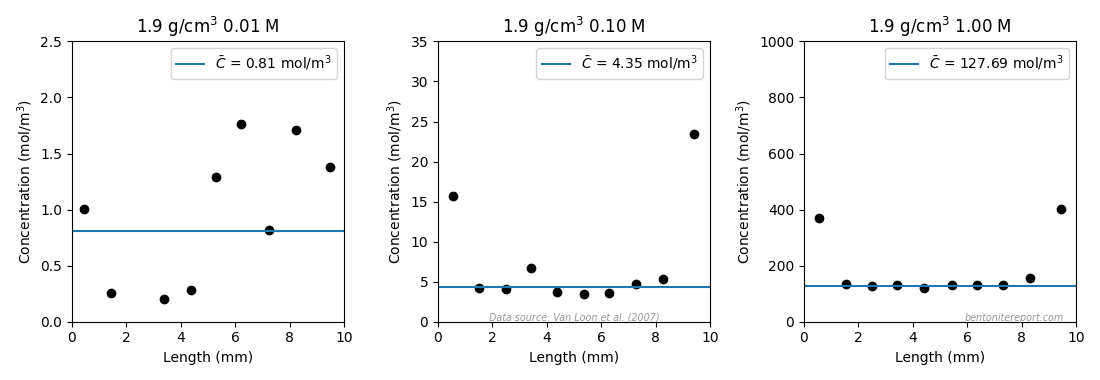
The chloride concentration increases near the interfaces in all samples; we have discussed this interface excess effect in previous posts. Vl07 deal with this issue by evaluating the averages only for the inner parts of the samples. I performed a similar evaluation, also presented in the above figures (blue lines). In this evaluation I adopted the criterion to exclude all points situated less than 2 mm from the interfaces (Vl07 seem to have chosen points a bit differently). The clay concentration reevaluated in this way is also listed in the above table (last column). Given that I have only used nominal density for each sample (I don’t have information on the actual density of the sample sections), I’d say that the re-evaluated values agree well with those de-derived from reported \(\epsilon_\mathrm{eff}\). One exception is the sample 1.9/0.01, which is seen to have concentration points all over the place (or maybe detection limit is reached?). While Vl07 choose the lowest three points in their evaluation, here we choose to discard this result altogether. I mean that it is rather clear that this concentration profile cannot be considered to represent equilibrium.
As the reevaluation gives similar values as those reported, and since we lack information for a full analysis, we will use the values de-derived from reported \(\epsilon_\mathrm{eff}\) in the continued assessment (except for sample 1.9/0.01).
Diffusion related estimations
Vl07 determine diffusion parameters by fitting various mathematical expressions to flux data.4 Parameters fitted in this way generally depend on the underlying adopted model, and we have discussed how equilibrium concentrations can be extracted from such parameters in an earlier blog post. In Vl07 it is clear that the adopted mathematical and conceptual model is the effective porosity diffusion model. When first presented in the article, however, it is done so in terms of a sorption distribution coefficient (\(R_d\)) that is claimed to take on negative values for anions. The presented mathematical expressions therefore contain a so-called rock capacity factor, \(\alpha\), which relates to \(R_d\) as \(\alpha = \phi + \rho_d\cdot R_d\). But such use of a rock capacity factor is a mix-up of incompatible models that I have criticized earlier. However, in Vl07 the description involving a sorption coefficient is in words only — \(R_d\) is never brought up again — and all results are reported, interpreted and discussed in terms of effective (or “chloride-accessible”) porosity, labeled \(\epsilon\) or \(\epsilon_\mathrm{Cl}\). We here exclusively use the label \(\epsilon_\mathrm{eff}\) when referring to formulas in Vl07. The mathematics is of course the same regardless if we call the parameter \(\alpha\), \(\epsilon\), \(\epsilon_\mathrm{Cl}\), or \(\epsilon_\mathrm{eff}\).
Mass balance in the out-diffusion stage
Vl07 measured the amount of tracers accumulated in the two reservoirs during the out-diffusion stage. The flux into the left side reservoir, which served as source reservoir during the preceding through-diffusion stage, was completely obscured by significant amounts of tracers present in the confining filter, and will not be considered further (also Vl07 abandon this flux in their analysis). But the total amount of tracers accumulated in the right side reservoir, \(N_\mathrm{right}\),5 can be used to directly estimate the chloride equilibrium concentration.
The initial concentration profile in the out-diffusion stage is linear (it is the steady-state profile), and the total amount of tracers, \(N_\mathrm{tot}\),6 can be expressed
\begin{equation} N_\mathrm{tot} = \frac{\phi\cdot \bar{c}_0\cdot V_\mathrm{sample}} {2} \tag{3} \end{equation}
where \(\bar{c}_0\) is the initial clay concentration at the left side interface, and \(V_\mathrm{sample}\) (\(\approx\) 5 cm3) is the sample volume.
A neat feature of the out-diffusion process is that two thirds of the tracers end up in the left side reservoir, and one third in the right side reservoir, as illustrated in this simulation

\(\bar{c}_0\) can thus be estimated by using \(N_\mathrm{tot} = 3\cdot N_\mathrm{right}\) in eq. 3, giving
\begin{equation} \frac{\bar{c}_0}{c_\mathrm{source}} = \frac{6 \cdot N_\mathrm{right}} {\phi \cdot V_\mathrm{sample}\cdot c_\mathrm{source}} \tag{4} \end{equation}
where \(c_\mathrm{source}\) is the tracer concentration in the left side reservoir in the through-diffusion stage.7 Although eq. 4 depends on a particular solution to the diffusion equation, it is independent of diffusivity (the diffusivity in the above simulation is \(1\cdot 10^{-10}\) m2/s). Eq. 4 can in this sense be said to be a direct estimation of \(\bar{c}_0\) (from measured \(N_\mathrm{right}\)), although maybe not as “direct” as the measurement of stable chloride, discussed previously.
Vl07 state eq. 4 in terms of a “Cl-accessible porosity”, but this is still just an interpretation of the clay concentration; \(\bar{c}_0\) is, in contrast to \(\epsilon_\mathrm{eff}\), directly accessible experimentally in principle. From the reported values of \(\epsilon_\mathrm{eff}\) we may back-calculate \(\bar{c}_0\), using the relation \(\bar{c}_0 / c_\mathrm{source} = \epsilon_\mathrm{eff}/\phi\). Alternatively, we may use eq. 4 directly to evaluate \(\bar{c}_0\) from the reported values of \(N_\mathrm{right}\). Curiously, these two approaches result in slightly different values for \(\bar{c}_0/c_\mathrm{source}\). I don’t understand the cause for this difference, but since \(N_\mathrm{right}\) is what has actually been measured, we use these values to estimate \(\bar{c}_0.\) The resulting equilibrium concentrations are
| Test | \(N_\mathrm{right}\) (10-10 mol) | \(\bar{c}_0/c_\mathrm{source}\) (-) |
| 1.3/0.01 | 4.10 | 0.038 |
| 1.3/0.05 | 10.2 | 0.097 |
| 1.3/0.1 | 17.8 | 0.168 |
| 1.3/0.4 | 41.4 | 0.395 |
| 1.3/1.0 | 52.4 | 0.445 |
| 1.6/0.01 | 1.21 | 0.014 |
| 1.6/0.05 | 3.64 | 0.043 |
| 1.6/0.1 | 6.15 | 0.072 |
| 1.6/0.4 | 13.0 | 0.154 |
| 1.6/1.0 | 21.6 | 0.225 |
| 1.9/0.01 | 0.41 | 0.006 |
| 1.9/0.05 | 1.14 | 0.018 |
| 1.9/0.1 | 1.64 | 0.025 |
| 1.9/0.4 | 3.19 | 0.051 |
| 1.9/1.0 | 8.19 | 0.113 |
We have now investigated two independent estimations of the chloride equilibrium concentrations: from mass balance of chloride tracers in the out-diffusion stage, and from measured stable chloride content. Here are plots comparing these two estimations

The similarity is quite extraordinary! With the exception of two samples (1.3/0.4 and 1.9/0.1), the equilibrium chloride concentrations evaluated in these two very different ways are essentially the same. This result strongly confirms that the evaluations are adequate.
Steady-state fluxes
Vl07 present the flux evolution in the through-diffusion stage only for a single test (1.6/1.0), and it looks like this (left diagram)

The outflux reaches a relatively stable value after about 7 days, after which it is meticulously monitored for a quite long time period. The stable flux is not completely constant, but decreases slightly during the course of the test. We anyway refer to this part as the steady-state phase, and to the preceding part as the transient phase.
One reason that the steady-state is not completely stable is, reasonably, that the source reservoir concentration slowly decreases during the course of the test. The estimated drop from this effect, however, is only about one percent,8 while the recorded drop is substantially larger, about 7%. Vl07 do not comment on this perhaps unexpectedly large drop, but it may be caused e.g. by the ongoing conversion of the bentonite to a purer sodium state (see above).
Most of the analysis in Vl07 is based on anyway assigning a single value to the steady-state flux. Judging from the above plot, Vl07 seem to adopt the average value during the steady-state phase, and it is clear that the assigned value is well constrained by the measurements (the drop is a second order effect). The steady-state flux can therefore be said to be directly measured in the through-diffusion stage, rather than being obtained from fitting a certain model to data.
Vl07 only implicitly consider the steady-state flux, in terms of a fitted “effective diffusivity” parameter, \(D_e\) (more on this in the next section). We can, however, “de-derive” the corresponding steady-state fluxes using \(j_\mathrm{ss} = D_e\cdot c_\mathrm{source}/L\), where \(L\) (= 0.01 m) is sample length. When comparing different tests it is convenient to use the normalized steady state flux \(\widetilde{j}_\mathrm{ss} = j_\mathrm{ss}/c_\mathrm{source}\), which then relates to \(D_e\) as \(\widetilde{j}_\mathrm{ss} = D_e/L\). Indeed, “effective diffusivity” is just a scaled version of the normalized steady-state flux, and it makes more sense to interpret it as such (\(D_e\) is not a diffusion coefficient). From the reported values of \(D_e\) we obtain the following normalized steady-state fluxes (my apologies for a really dull table)
| Test | \(D_e\) (10-12 m2/s) | \(\widetilde{j}_\mathrm{ss}\) (10-10 m/s) |
| 1.3/0.01 | 2.6 | 2.6 |
| 1.3/0.05 | 7.5 | 7.5 |
| 1.3/0.1 | 16 | 16 |
| 1.3/0.4 | 25 | 25 |
| 1.3/1.0 | 49 | 49 |
| 1.6/0.01 | 0.39 | 0.39 |
| 1.6/0.05 | 1.1 | 1.1 |
| 1.6/0.1 | 2.3 | 2.3 |
| 1.6/0.4 | 4.6 | 4.6 |
| 1.6/1.0 | 10 | 10 |
| 1.9/0.01 | 0.033 | 0.033 |
| 1.9/0.05 | 0.12 | 0.12 |
| 1.9/0.1 | 0.24 | 0.24 |
| 1.9/0.4 | 0.5 | 0.5 |
| 1.9/1.0 | 1.2 | 1.2 |
Plotting \(\widetilde{j}_\mathrm{ss}\) as a function of background concentration gives the following picture

The steady-state flux show a very consistent behavior: for all three densities, \(\widetilde{j}_\mathrm{ss}\) increases with background concentration, with a higher slope for the three lowest background concentrations, and a smaller slope for the two highest background concentrations. Although we have only been able to investigate the 1.6/1.0 test in detail, this consistency confirms that the steady-state flux has been reliably determined in all tests.
Transient phase evaluations
So far, we have considered estimations based on more or less direct measurements: stable chloride concentration profiles, tracer mass balance in the out-diffusion stage, and steady-state fluxes. A major part of the analysis in Vl07, however, is based on fitting solutions of the diffusion equation to the recorded flux.
Vl07 state somewhat different descriptions for the through- and out-diffusion stages. For out-diffusion they use an expression for the flux into the right side reservoir (the sample is assumed located between \(x=0\) and \(x=L\))
\begin{equation} j(L,t) = -2\cdot j_\mathrm{ss} \sum_{n = 1}^\infty \left(-1\right )^n\cdot e^{-\frac{D_e\cdot n^2\cdot \pi^2\cdot t} {L^2\cdot \epsilon_\mathrm{eff}}} \tag{5} \end{equation}
where \(j_\mathrm{ss}\) is the steady-state flux,9 \(D_e\) is “effective diffusivity”, and \(\epsilon_\mathrm{eff}\) is the effective porosity parameter (Vl07 also state a similar expression for the diffusion into the left side reservoir, but these results are discarded, as discussed earlier). For through-diffusion, Vl07 instead utilize the expression for the amount tracer accumulated in the right side reservoir
\begin{equation} A(L,t) = S\cdot L \cdot c_\mathrm{source} \left ( \frac{D_e\cdot t}{L^2} – \frac{\epsilon_\mathrm{eff}} {6} – \frac{2\cdot\epsilon_\mathrm{eff}}{\pi^2} \sum_{n = 1}^\infty \frac{\left(-1\right )^n}{n^2} \cdot e^{-\frac{D_e\cdot n^2\cdot \pi^2\cdot t} {L^2\cdot \epsilon_\mathrm{eff}} }\right ) \tag{6} \end{equation}
were \(S\) denotes the cross section area of the sample.
It is clear that Vl07 use \(D_e\) and \(\epsilon_\mathrm{eff}\) as fitting parameters, but not exactly how the fitting was conducted. \(D_e\) seems to have been determined solely from the the through-diffusion data, while separate values are evaluated for \(\epsilon_\mathrm{eff}\) from the through- and out-diffusion stages. As already discussed, Vl07 also provide a third estimation of \(\epsilon_\mathrm{eff}\), based on mass-balance in the out-diffusion stage. To me, the study thereby gives the incorrect impression of providing a whole set of independent estimations of \(\epsilon_\mathrm{eff}\). Although eqs. 5 and 6 are fitted to different data, they describe diffusion in one and the same sample, and an adequate fitting procedure should provide a consistent, single set of fitted parameters \((D_e, \epsilon_\mathrm{eff})\). Even more obvious is that the estimation of \(\epsilon_\mathrm{eff}\) from fitting eq. 5 should agree with the estimation from the mass-balance in the out diffusion stage — the accumulated amount in the right side reservoir is, after all, given by the integral of eq. 5. A significant variation of the reported fitting parameters for the same sample would thus signify internal inconsistency (experimental- or modelwise).
In the following reevaluation we streamline the description by solely using fluxes as model expressions,4 and by emphasizing steady-state flux as a parameter, which I think gives particularly neat expressions,10 (“TD” and “OD” denote through- and out-diffusion, respectively)
\begin{equation} \widetilde{j}_{TD}(L,t) = \widetilde{j}_\mathrm{ss} \left ( 1 + 2 \sum_{n = 1}^\infty \left(-1\right )^n \cdot e^{-\frac{D_p\cdot n^2\cdot \pi^2\cdot t} {L^2} }\right ) \tag{7} \end{equation}
\begin{equation} \widetilde{j}_{OD}(L,t) = -2\cdot \widetilde{j}_\mathrm{ss} \sum_{n = 1}^\infty \left( -1 \right )^n \cdot e^{-\frac{D_p\cdot n^2\cdot \pi^2\cdot t} {L^2}} \tag{8} \end{equation}
Here we use the pore diffusivity, \(D_p\), instead of the combination \(D_e/\epsilon_\mathrm{eff}\) in the exponential factors, and \(\widetilde{j} = j/c_\mathrm{source}\) denotes normalized flux. This formulation clearly shows that the time evolution is governed solely by \(D_p\), and that \(\widetilde{j}_\mathrm{ss}\) simply acts as a scaling factor.
In my opinion, using \(\widetilde{j}_\mathrm{ss}\) and \(D_p\) gives a formulation more directly related to measurable quantities; the steady-state flux is directly accessible experimentally, as we just examined, and \(D_p\) is an actual diffusion coefficient (in contrast to \(D_e\)) that can be directly evaluated from clay concentration profiles. Of course, eqs. 7 and 8 provide the same basic description as eqs. 5 and 6, and \(\widetilde{j}_\mathrm{ss}\) and \(D_p\) are related to the parameters reported in Vl07 as
\begin{equation} \widetilde{j}_\mathrm{ss} = \frac{D_e}{L} \tag{9} \end{equation}
\begin{equation} D_p = \frac{D_e}{\epsilon_\mathrm{eff}} \tag{10} \end{equation}
When reevaluating the reported data we focus on the above discussed consistency aspect, i.e. whether or not a single model (a single pair of parameters) can be satisfactory fitted to all available data for the same sample. In this regard, we begin by noting that the fitting parameters are already constrained by the direct estimations. We have already concluded that the recorded steady-state flux basically determines \(\widetilde{j}_\mathrm{ss}\), and if we combine this with the estimated chloride clay concentration, \(D_p\) is determined from \(j_\mathrm{ss} = \phi\cdot D_p\cdot \bar{c}_0/L\), i.e.
\begin{equation} D_p = \frac{\widetilde{j}_\mathrm{ss}\cdot L} {\phi\cdot \left (\bar{c}_0 / c_\mathrm{source}\right )} \tag{11} \end{equation}
Here are plotted values of \(D_p\) evaluated in this manner

Note that these values basically remain constant for samples of similar density (within a factor of 2) as the background concentration is varied by two orders of magnitude. This is the expected behavior of an actual diffusion coefficient,11 and confirms the adequacy of the evaluation; the numerical values also compares rather well with corresponding values for “MX-80” bentonite, measured in closed-cell tests (indicated by dashed lines in the figure).
Using eq. 10, we can also evaluate values of \(D_p\) corresponding to the various reported fitted parameters \(\epsilon_\mathrm{eff}\). The result looks like this (compared with the above evaluations from direct estimations)

As pointed out above, a consistent evaluation requires that the parameters fitted to the out-diffusion flux (red) are very similar to those evaluated from considering the mass balance in the same process (blue). We note that the resemblance is quite reasonable, although some values — e.g. tests 1.3/1.0 and 1.6/1.0 — deviate in a perhaps unacceptable way.
\(D_p\) evaluated from reported through-diffusion parameters, on the other hand, shows significant scattering (green). As the rest of the values are considerably more collected, and as the steady-state fluxes show no sign whatsoever that the diffusion coefficient varies in such erratic manner, it is quite clear that this scattering indicates problems with the fitting procedure for the through-diffusion data.
The 1.6/1.0 test
To further investigate the fitting procedures, we take a detailed look at the 1.6/1.0 test, for which flux data is provided. Vl07 report fitted parameters \(D_e = 1.0\cdot 10^{-11}\) m2/s and \(\epsilon_\mathrm{eff} = 0.063\) to the through-diffusion data, corresponding to \(\widetilde{j}_\mathrm{ss} = 1.0\cdot 10^{-9}\) m/s and \(D_p = 1.6\cdot 10^{-10}\) m2/s. We have already concluded that the steady-state flux is well captured by this data, but to see how well fitted \(\epsilon_\mathrm{eff}\) (or \(D_p\)) is, lets zoom in on the transient phase

This diagram also contains models (eq. 7) with different values of \(D_p\), and with a slightly different value of \(j_\mathrm{ss}\).12 It is clear that the model presented in the paper (black) completely misses the transient phase, and that a much better fit is achieved with \(D_p = 9.7\cdot10^{-11}\) m2/s (and \(\widetilde{j}_\mathrm{ss} = 1.06\cdot 10^{-9}\) m/s) (red). This difference cannot be attributed to uncertainty in the parameter \(D_p\) — the reported fit is simply of inferior quality. With that said, we note that all information on the transient phase is contained within the first three or four flux points; the reliability could probably have been improved by measuring more frequently in the initial stage.13
A reason for the inferior fit may be that Vl07 have focused only on the linear part of eq. 6; the paper spends half a paragraph discussing how the approximation of this expression for large \(t\) can be used to extract the fitting parameters using linear regression. Does this mean that only experimental data for large times where used to evaluate \(D_e\) and \(\epsilon_\mathrm{eff}\)? Since we are not told how fitting was performed, we cannot answer this question. Under any circumstance, the evidently low quality of the fit puts in question all the reported \(\epsilon_\mathrm{eff}\) values fitted to through-diffusion data. This is actually good news, as several of the corresponding \(D_p\) values were seen to be incompatible with constraints from direct estimations. We can thus conclude with some confidence that the inconsistency conveyed by the differently evaluated fitting parameters does not indicate experimental shortcomings, but stems from bad fitting of the through-diffusion model. Therefore, we simply dismiss the reported \(\epsilon_\mathrm{eff}\) values evaluated in this way. Note that the re-fitted value for \(D_p\) \((9.7\cdot10^{-11}\) m2/s) is consistent with those evaluated from direct estimations.
We note that when fitting the transient phase, it is appropriate to use a value of \(\widetilde{j}_\mathrm{ss}\) slightly larger than the average value adopted by Vl07 (as the model does not account for the observed slight drop of the steady-state flux). This is only a minor variation in the \(\widetilde{j}_\mathrm{ss}\) parameter itself (from \(1.02\cdot10^{-9}\) to \(1.06\cdot10^{-9}\) m/s), but, since this value sets the overall scale, it indirectly influences the fitted value of \(D_p\) (model fitting is subtle!).
More questions arise regarding the fitting procedures when also examining the presented out-diffusion stage for the 1.6/1.0 sample. The tabulated fitted value for this stage is \(\epsilon_\mathrm{eff}\) = 0.075, while it is implied that the same value has been used for \(D_e\) as evaluated from the the through-diffusion stage (\(1.0\cdot 10^{-11}\) m2/s). The corresponding pore diffusivity is \(D_p = 1.33\cdot 10^{-10}\) m2/s. The provided plot, however, contains a different model than tabulated, and looks similar to this one (left diagram)
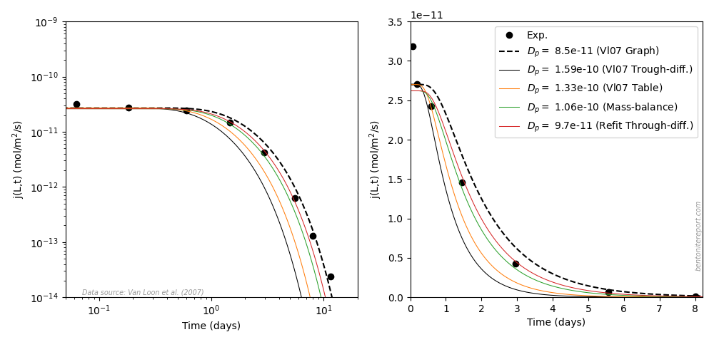
Here the presented model (black dashed line) instead corresponds to \(D_p = 8.5\cdot 10^{-11}\) m2/s (or \(\epsilon_\mathrm{eff}\) = 0.118). The model corresponding to the tabulated value (orange) does not fit the data! I guess this error may just be due to a typo in the table, but it nevertheless gives more reasons to not trust the reported \(\epsilon_\mathrm{eff}\) values fitted to diffusion data.
The above diagram also shows the model corresponding to the reported parameters from the through-diffusion stage (black solid line). Not surprisingly, this model does not fit the out-diffusion data, confirming that it does not appropriately describe the current sample. The model we re-fitted in the through-diffusion stage (red), on the other hand, captures the outflux data quite well. By also slightly adjusting \(\widetilde{j}_{ss}\), from from \(1.06\cdot10^{-9}\) to \(0.99\cdot10^{-9}\) m/s, to account for the drop in steady-state flux during the course of the through-diffusion test, and by plotting in a lin-lin rather than a log-log diagram, the picture looks even better! In a lin-lin plot (right diagram), it is easier to note that the model presented in the graph of Vl07 actually misses several of the data points. Could it be that Vl07 used visual inspection of the model in a log-log diagram to assess fitting quality? If so, data points corresponding to very low fluxes are given unreasonably high weight.14 This could be (another) reason for the noted difference between \(D_p\) evaluated from fitted parameters to the out-diffusion flux, and from the total accumulated amount of tracer (which should be equal).
From examining the reported results of sample 1.6/1.0 we have seen that the fitting procedures adopted in Vl07 appear inappropriate, but also that a consistent model can be successfully fitted to all available data (using a single \(D_p\)). Vl07 don’t provide flux data for any other sample, but we must conclude that the reported fitted \(\epsilon_\mathrm{eff}\) parameters cannot be trusted. Luckily, the preformed refitting exercise confirms the results obtained from analysis of stable chloride profiles and accumulated amount of tracers in out-diffusion, and we conclude that these results most probably are reliable. The corresponding value of \(\bar{c}_0/c_\mathrm{source}\) (using eq. 11) for the refitted model is here compared with the estimations from direct measurements

Summary and verdict
Chloride equilibrium concentrations evaluated from mass balance of the tracer in the out-diffusion stage and from stable chloride content show remarkable agreement. On the other hand, the scattering of estimated concentrations increases substantially if they are also evaluated from the reported fitted diffusion parameters. This could indicate underlying experimental problems, as a consistent evaluation should result in a single value for the equilibrium concentration; the various evaluations — stable chloride, out-diffusion mass balance, through-diffusion fitting and out-diffusion fitting — relate, after all, to a single sample.
By reexamining the evaluations we have found, however, that the problem is associated with how the fitting to diffusion data has been conducted (and presented), rather than indicating fundamental experimental issues. In the test that we have been able to examine in detail (1.6/1.0), we found that the reported models do not fit data, but also that it is possible to satisfactorily refit a single model that is also compatible with the direct methods for evaluating the equilibrium concentration. For the rest of the samples, we have also been able to discard the fitted diffusion parameters, as they are not compatible e.g. with how the steady-state flux (very consistently) vary with density and background concentration.
For these reasons, we discard the reported “effective porosity” parameters evaluated from fitting solutions of the diffusion equation to flux data, and keep the results from direct measurements of chloride equilibrium concentrations (from stable chloride profile analysis and mass-balance in the out-diffusion stage). I judge the resulting chloride equilibrium concentrations as reliable and that they can be used for increased qualitative process understanding. I furthermore judge the directly measured steady-state fluxes as reliable. This study thus provide adequate values for both chloride equilibrium concentrations and diffusion coefficients.
However, a frustrating problem is that, although the equilibrium concentrations are well determined, we have little information on the exact state of the samples in which they have been measured. We basically have to rely on that the “KWK” material is “similar” to “MX-80”, keeping in mind that “MX-80” is not really a uniform material (from a scientific point of view). Also, the exchangeable mono/divalent cation ratio is most probably quite different in samples contacted with different background concentrations.
Yet, I judge the present study to provide the best information available on chloride equilibrium in compacted bentonite, and will use it e.g. for investigating the salt exclusion mechanism in these systems (I already have). That this information is the best available is, however, also a strong argument for that more and better constrained data is urgently needed.
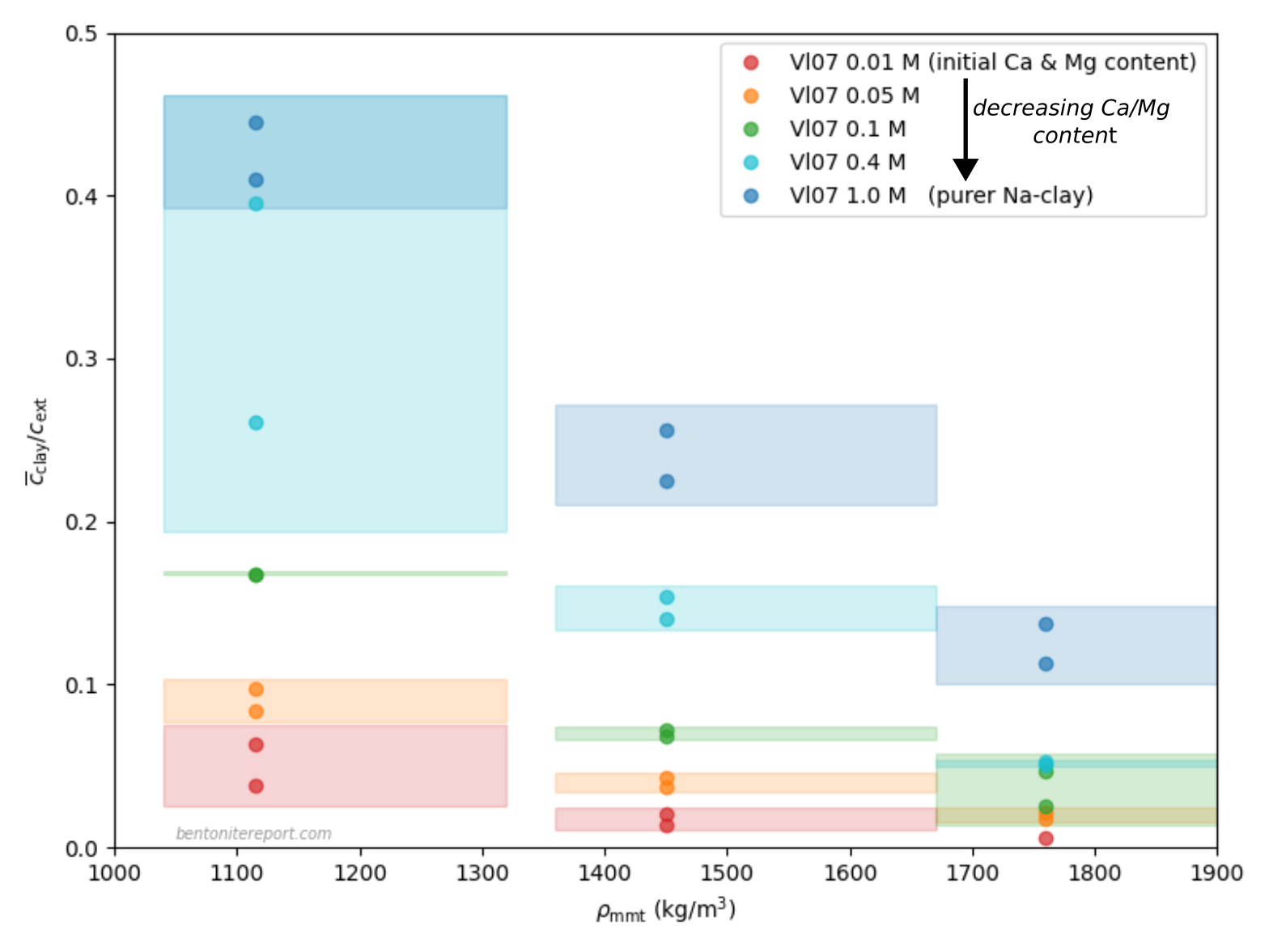
The (reliable) results are presented in the diagram below, which includes “confidence areas”, that takes into account the spread in equilibrium concentrations, in samples where more than a single evaluation were performed, and the estimated uncertainty in effective montmorillonite dry density (the actual points are plotted at nominal density, assuming 80% montmorillonite content)
- Chloride content: UNKNOWN
- Extracting anion equilibrium concentrations from through-diffusion tests
- Assessment of chloride equilibrium concentrations: Muurinen et al. (1988)
- Assessment of chloride equilibrium concentrations: Molera et al. (2003)
- How salt equilibrium concentrations may be overestimated
- Assessment of chloride equilibrium concentrations: Muurinen et al. (2004)
Footnotes
[1] Vejsada et al. (2006) call their material “KWK 20-80”. In other contexts, I have also found the versions “KWK food grade” and “KWK krystal klear”. I have given up my attempts at trying to understand the difference between these “KWK” variants.
[2] Van Loon et al. (2007) label the background concentration \([\mathrm{Cl}]_0\).
[3] This should be relatively straightforward, but I get at bit nervous e.g. about the presence of a rather arbitrary factor 0.85 in the presented formula (eq. 19 in Van Loon et al. (2007)).
[4] As always for these types of diffusion tests, the raw data consists of simultaneously measured values of time (\(\{t_i\}\)) and reservoir concentrations (\(\{c_i\}\)). From these, flux can be evaluated as (\(A\) is sample cross sectional area, and \(V_\mathrm{res}\) is reservoir volume)
\begin{equation} \bar{j}_i = \frac{1}{A} \frac{ \left (c_i – c_{i-1} \right ) \cdot V_\mathrm{res}} {t_i – t_{i-i}} \tag{*} \end{equation}
\(\bar{j}_i\) is the mean flux in the time interval between \(t_{i-1}\) and \(t_i\), and should be associated with the average time of the same interval: \(\bar{t}_i = (t_i + t_{i-1})/2\). The above formula assumes no solution replacement after the \((i-1)\):th measurement (if the solution is replaced, \(\left (c_i – c_{i-1} \right )\) should be replaced with \(c_i\)).
Alternatively one can work with the accumulated amount of substance, which e.g. is \(N(t_i) = \sum_{j=1}^i c_j\cdot V_\mathrm{res}\), in case the solution is replaced after each measurement. I prefer using the flux because eq. * only depends on two consecutive measurements, while \(N(t_i)\) in principle depends on all measurements up to time \(t_i\). Also, I think it is easier to judge how well e.g. a certain model fits or is constrained by data when using fluxes; the steady-state, for example, then corresponds to a constant value.
Van Loon et al. (2007) seem to have utilized both fluxes and accumulated amount of substance in their evaluations, as discussed in later sections.
[5] Van Loon et al. (2007) denote this quantity \(A(L)\).
[6] Van Loon et al. (2007) denote this quantity \(A_w\), \(A_\mathrm{out}\), and \(A_\mathrm{tot}\).
[7] Van Loon et al. (2007) denote this quantity \(C_0\).
[8] From total test time, recorded flux, and sample cross sectional area, we estimate that about \(5.8\cdot 10^{-8}\) mol of tracer is transferred from the source reservoir during the course of the test (\(50\) days\(\cdot 2.7\cdot 10^{-11}\) mol/m2/s\(\cdot 0.0005\) m2). This is about 1% of the total amount tracer, \(c_\mathrm{source} \cdot V_\mathrm{source} = 2.65 \cdot 10^{-5}\) M \(\cdot 0.2\) L = \(5.3\cdot 10^{-6}\) mol.
[9] Van Loon et al. (2007) label this parameter \(J_L\), and don’t relate it explicitly to the steady-state flux. From the experimental set-up it is clear, however, that the initial value of the out-diffusion flux (into the right side reservoir) is the same as the previously maintained steady-state flux. Note that the expressions for the fluxes in the out-diffusion stage in Van Loon et al. (2007) has the wrong sign.
[10] The description provided by eqs. 5 and 6 not only mixes expressions for flux and accumulated amount tracer, but also contains three dependent parameters \(D_e\), \(\epsilon_\mathrm{eff}\), and \(j_\mathrm{ss}\) (e.g. \(j_\mathrm{ss} = D_e/(c_\mathrm{source}\cdot L)\)). In this reformulation, the model parameters are strictly only \(\widetilde{j}_\mathrm{ss}\) and \(D_p\). We have also divided out \(c_\mathrm{source}\) to obtain equations for normalized fluxes. Note that the expression for \(\widetilde{j}_{TD}(L,t)\) is essentially the same that we have used in previous assessments of through-diffusion tests. Note also that eqs. 7 and 8 imply the relation \(\widetilde{j}_{OD}(L,t) = \widetilde{j}_{ss} – \widetilde{j}_{TD}(L,t)\), reflecting that the out-diffusion process is essentially the through-diffusion process in reverse.
[11] Note the similarity with that diffusivity also is basically independent of background concentration for simple cations. Note also that there is no reason to expect completely constant \(D_p\) for a given density, because the samples are not identically prepared (being saturated with saline solutions of different concentration).
[12] As we here consider a single sample, we alternate a bit sloppily between steady-state flux (\(j_\mathrm{ss} \)) and normalized steady-state flux (\(\widetilde{j}_\mathrm{ss}\)), but these are simply related by a constant: \(\widetilde{j}_\mathrm{ss} = j_\mathrm{ss} / c_\mathrm{source}\). For the 1.6/1.0 test this constant is (as tabulated) \(c_\mathrm{source} = 2.65\cdot 10^{-2}\) mol/m3.
[13] I think it is a bit amusing that the pattern of data points suggests measurements being performed on Mondays, Wednesdays, and Fridays (with the test started on a Wednesday).
[14] I have warned about the dangers of log-log plots earlier.