In a previous post I discussed how parts of the bentonite¹ research community unjustifiably explain variation in (effective) diffusion rates as changes in “diffusion paths”. But what do authors really mean when using the term “diffusion path”?

In the geochemical/reactive transport literature, “diffusive pathways” are usually introduced when discussing the (presumably) related concept of tortuosity. For example, Steefel and Maher (2009) present a figure very similar to the one below, with the caption “Tortuous diffusion paths in porous material.”

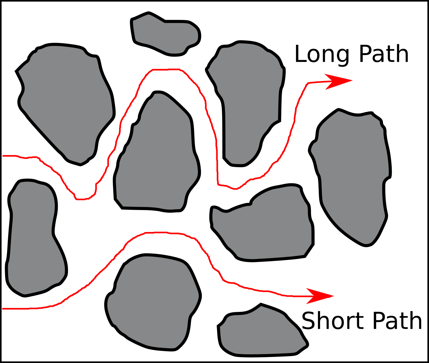
The text explains further that these are paths “the solute […] follow[s] in tortuous media”². Several questions immediately arise. For example:

• What is it, exactly, that follows these paths?
• Why do the paths have a direction?
• Why are these particular paths singled out? What stops e.g. the “Long Path” from taking this obvious shortcut:

Let’s start with a hopefully obvious statement: Individual molecules or ions do not follow “paths” in a diffusive process, but conduct random motion. So paths as those in the figure above are certainly not trajectories of single particles.³

An answer to what is illustrated may be found in Van Brakel and Heertjes (1974) — a main reference in the bentonite research community when discussing tortuosity etc.⁴ In this work, the system is analyzed in steady-state, and the following description is given for “diffusion paths”

Assume the pore space of the porous medium to be completely filled with what we will call diffusion paths. The main direction of the diffusion paths is the same as that of the concentration gradient. In the way the diffusion paths wind through the pore space they can be compared with the streamlines for laminar flow in porous media.

Here it may sound as if the authors reject Fickian diffusion (which is always parallel to the concentration gradient), but it is rather that they use the term “concentration gradient” for denoting the externally applied constant concentration difference, required to maintain a steady-state flux. To me, this is quite confusing, because the comparison of diffusion paths with streamlines implies that they are directed along a (negative) concentration gradient. Two “gradients” must thus be kept in mind simultaneously: the external concentration difference, and the actual gradient on the pore-scale.

But with this distinction made, it is clear what Van Brakel and Heertjes mean by “diffusion paths”, and that their aim is to reduce a more complex 3D problem to an effective 1D description. It also becomes relatively clear that this is the way the term is used in much of the bentonite literature. It explains e.g. why the “paths” in the above picture (and others) have a direction: they must be thought of as the steady-state flow on the pore scale, with an implied constant concentration difference applied across the sample, making the macroscopic flow effectively 1D.

This implied reduction to steady-state transport in 1D is often found in the literature, e.g. in Shackelford and Moore (2013)

This increased tortuosity reduces the macroscopic concentration gradient (i.e., increases the distance over which the concentration difference is applied) and, therefore, reduces the diffusive mass flux relative to that which would exist in the absence of the porous medium.

or in Altman et al. (2015)

\(\tau\) is a geometrical factor (\(\le 1\)) representing the reduction in the effective concentration gradient (d(Me)/dx) due to the fact that diffusion paths through a porous medium will generally be greater, i.e. more tortuous, than the straight-line distance between the system boundaries, i.e. dx.

I am quite puzzled by this description for several reasons. Firstly, I find it unsatisfying that these definitions require the system to be in steady-state. Information on the influence of geometry is of course contained in the diffusion coefficient itself, independent of any external concentration differences. To associate “tortuosity” with such concentration differences, rather than with the mobility of the diffusing substance, seems inadequate to me. Moreover, the procedure of reducing a “macroscopic” concentration gradient due to path length seems to only work for an isolated path. At least, the procedure must become more involved for a system of connected paths, something I’ve not seen commented on by authors adopting this concept.

Secondly, note that a “diffusion path” — with the steady-state definition — simply indicates net mass transfer of diffusing substance. The absence of a “diffusion path” in a region does not mean that dissolved constituents don’t migrate there, but only that flux contributions in different directions add up to zero net mass transfer. I did a silly random walk simulation to illustrate this point (the concentration of walkers is kept at a constant finite value on the left side of the domain, while it is kept at zero on the right side)

Note that with the definitions here discussed, we must accept that the vertical section in this illustration is not a diffusion path. This situation is quite distinct from laminar advective transport, where — if I’m thinking correctly — the absence of a streamline implies the absence of motion.

Thirdly, if you consider a porous system to be a network of thin cylinders, I guess the steady-state flux will basically resemble the the system itself (interconnected 1D-spaghetti configured in 3D). I suspect that this is the view many authors have in mind when speaking of “diffusion paths”. But, if so, why not simply speak of “paths”? Note also that the pore volume of smectitic systems mainly consists of 2D water films configured in 3D (it is lasagna, not spaghetti).

Lastly, what about non-steady-state transport? Concepts like the ones discussed here are also used when describing closed-cell diffusion tests , but are seldom (never?) defined in any other way. How could e.g. “tortuosity” reduce a macroscopically applied (1D) gradient in this case? And what is even meant by “diffusion paths”, if these are defined in steady-state? Since non-steady state is the general case, it would be more satisfying if quantities obtained under such circumstances were applied to the steady-state, rather than the other way around.

To get a feel for how pore geometry influences diffusion in non-steady-state, I conducted some more random walk simulations. In the animation below is compared random walks in an unrestricted 2D plane (blue) with random walks on a square net (red; strip width: 1 length unit, square size: 20 length units)

To quantify the diffusivity, we plot the average of the square of the displacements, \(\langle r^2 \rangle\), as a function of time⁵ in the two systems

We see that the diffusivity — which is directly proportional to the slope of these curves — is very close to twice as large in the unrestricted case as compared with diffusion on the net. From such a result it may be tempting to conclude that this reduction by a factor of two is due to longer “diffusion paths” on the net (and relate it to \(\sqrt{2}\), which conveniently is the ratio between the side and the diagonal of a square). But note that the diffusional process is isotropic also on the net, as demonstrated by identical slopes of the angle-resolved \(\langle r^2 \rangle\)-curves. Thus, interpreted in terms of “diffusion paths” on the net — however these should be defined — the conclusion is that the “paths” have the same length in any direction.

But the situation is easily analyzed from the simple model underlying the figures displayed above: in the 2D-plane, the random walk process has a maximized variance, because movements in the \(x-\) and \(y-\)directions are uncorrelated. The net geometry, on the other hand, correlates these variables: if a walker has free passage in the \(y\)-direction, it is restricted in the \(x\)-direction, and vice versa. Thus, the diffusivity is not diminished due to longer “paths”, but because the geometrical restrictions reduce the variance of the underlying process. This effect will depend on the relative reduction of dimensions: with line-like pores in a 3D configuration, the reduction factor becomes 1/3 (I guess this is what what is alluded to for a “homogeneous isotropic pore network” in the often-cited work Dykhuzien and Casey (1989) ), but for the case relevant for bentonite — diffusion in 2D-planes configured in 3D — the factor is 2/3 (which I haven’t seen stated anywhere). I furthermore don’t understand why such a factor should be termed “tortuosity”, because there is nothing intrinsically “tortuous” about it (in a sense one could even argue that individual trajectories in the unrestricted 2D-plane are more “tortuous” than the ones on the net).

By making the net non-isotropic, e.g. by replacing the squares by rectangles like this

the correlation between the \(x\)- and \(y\)-variables alters (it is now twice as likely for a walker to have no restriction in the \(y\)-direction as in the \(x\)-direction), which is directly reflected in the diffusivities

The diffusivity in the \(y\)-direction is now about twice as large as the diffusivity in the \(x\)-direction. Also the diffusivity in the diagonal directions is significantly larger than in the \(x\)-direction. Following a naive definition of “tortuosity”, this result may seem surprising (is the “solute” in the \(x\)-direction following a longer path than than in the diagonal directions?). Still, with a correct averaging procedure I guess the diffusivity can be related to “paths” on the net (However, I still don’t understand how to differ “diffusion paths” from geometrical paths).

With these simulations I simply want to argue for that it seems considerably more subtle and complex to relate pore geometry to diffusivity, than how it typically is presented in the bentonite literature. To be frank, I consider most talk about “diffusion paths” in the bentonite literature, as well as most definitions of various geometric factors, to be just that: talk. There is an established “tradition” to mention certain concepts (geometric factors, tortuosity, constrictivity, paths…), but in the end the introduced factors are usually only functioning as fudge factors, leading to unjustified claims about the nature of bentonite. Similarly, discussions on actual values of such factors are in principle always only qualitative.

As an example, Choi and Oscarson (1996) interpret different values of diffusivity measured in Na- and Ca-bentonite directly as a difference in “tortuosity”:

We attribute this to the larger quasicrystal, or particle, size of Ca- compared to Na-bentonite. Hence, Ca-bentonite has a greater proportion of relatively large pores; this was confirmed by Hg intrusion porosimetry. This means the diffusion pathways in Ca-bentonite are less tortuous than those in Na-bentonite.

But they could have been considerably more quantitative than this. In the paper, tortuosity is defined as \(\tau = L^2/L_e^2\), where “\(L\) is the straight-line macroscopic distance between two points defining the transport path, and \(L_e\) is the actual, microscopic or effective distance between the same two points.” Tortuosity is furthermore evaluated from HTO diffusion to \(\tau_{\ce{Na}} = 0.062\) in Na-bentonite, and \(\tau_{\ce{Ca}} = 0.117\) in Ca-bentonite. Combining these expressions gives \(L_{e,\ce{Na}} = 1.37\cdot L_{e,\ce{Ca}}\).

What is implicitly said in this work is thus that the “actual, microscopic or effective distance between two points” is 1.37 times longer in Na-bentonite as compared with Ca-bentonite. I mean that it would be suitable for authors making these kind of (implicit) claims to provide a quantitative idea of how the pore space is modified in order to achieve this particular alteration of distances. To me, it is not even obvious why “larger quasicrystals” implies shorter “diffusion paths” — note that the effect of the “net” geometries above are scale independent.

But rather than making a quantitative discussion, Choi and Oscarson (1996) give the following caveat

In reality, \(\tau\) may account for more than just the pore geometry of the clay. Another factor that may be included in \(\tau\) is, for instance, the variation in the viscosity of the solution within the pore space (Kemper et al., 1964).

I find this an incredible statement. It is similar to saying that, “in reality”, Earth’s gravity constant (\(g\)) may include effects of air resistance.

Footnotes

[1] “Bentonite” is used in the following as an abbreviation of “Bentonite and claystone”.

[2] That is at least my interpretation. A fuller quotation reads: “[Tortuosity] is defined as the ratio of the path length the solute would follow in water alone, \(L\), relative to the tortuous path length it would follow in porous media, \(L_e\)” (while the following equation actually contains the square of this ratio).

[3] I am not fully convinced that all authors keep this in mind at all times. How should e.g. the following passage from Charlet et al. (2017) be interpreted: “An important geometric parameter is the tortuosity factor, \(\tau\), that quantifies the travelled distance of a dissolved constituent through the pore network compared to actual distance between two points.”? Or this one from Van loon et al. (2018) : “The tortuosity is a measure for path lengthening and takes into account that molecules have to diffuse around grains and thus take a longer way.”?

[4] Which is quite amazing, considering that this paper deals with diffusion in a gas phase in macroporous systems.

[5] Since all walkers start in the same point (the origin) the data show finite-size effects for small times. The presented data is therefore taken after an initiation time, labeled \(t^\star\).